import pandas as pd
import numpy as np
import matplotlib.pyplot as plt
import seaborn as sns
import xgboost as xgb
from sklearn.metrics import mean_squared_error
color_pal = sns.color_palette()
plt.style.use('fivethirtyeight')
df = pd.read_csv('AAPL Hourly.csv')
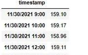
df = df[['timestamp', 'close']]df = df.set_index('timestamp')df.plot(style='.', figsize=(15, 5), color=color_pal[0], title='stock growth')
plt.show()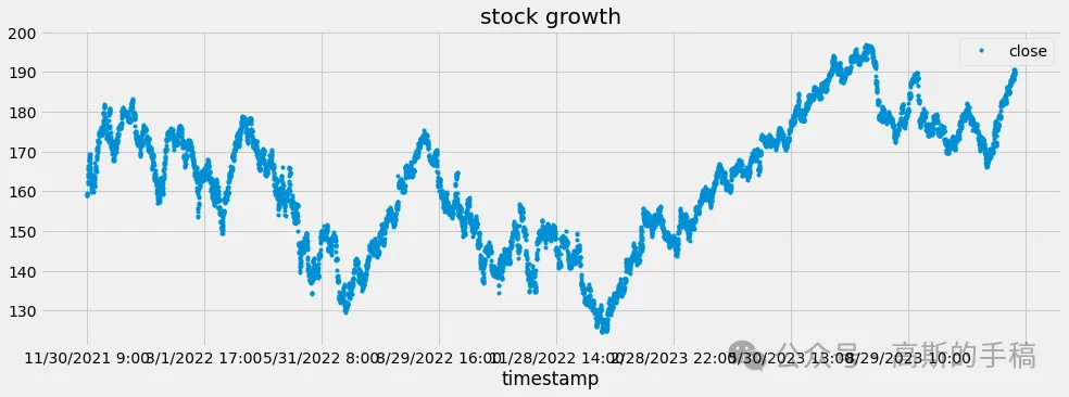
df.head()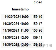
mean  = df['close'].mean()
mean162.3033402402023df.index = pd.to_datetime(df.index)Train / Test Split
train = df.loc[df.index < '01/01/2023']
test = df.loc[df.index >= '01/01/2023']
fig, ax = plt.subplots(figsize=(15, 5))
train.plot(ax=ax, label='Training Set', title='Data Train/Test Split')
test.plot(ax=ax, label='Test Set')
ax.axvline('01-01-2023', color='black', ls='--')
ax.legend(['Training Set', 'Test Set'])
plt.show()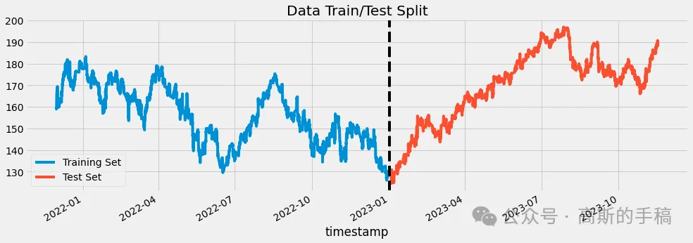
df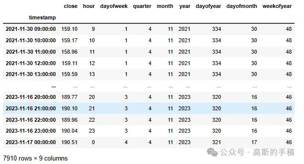
df.loc[(df.index > '01/01/2022') & (df.index < '01/08/2022')] \
    .plot(figsize=(15, 5), title='Week Of Data')
plt.show()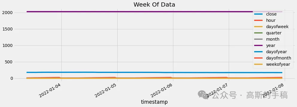
Feature Creation
def create_features(df):    """    Create time series features based on time series index.    """    df = df.copy()    df['hour'] = df.index.hour    df['dayofweek'] = df.index.dayofweek    df['quarter'] = df.index.quarter    df['month'] = df.index.month    df['year'] = df.index.year    df['dayofyear'] = df.index.dayofyear    df['dayofmonth'] = df.index.day    df['weekofyear'] = df.index.isocalendar().week    return df
df = create_features(df)
Visualize Our Feature / Target Relationship
fig, ax = plt.subplots(figsize=(10, 8))
sns.barplot(data=df, x='hour', y='close')
ax.set_title('price by hour')
plt.show()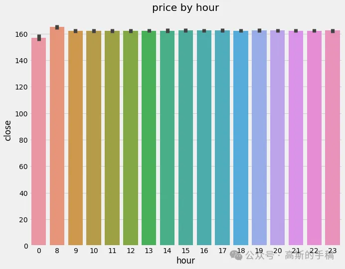
fig, ax = plt.subplots(figsize=(10, 8))
sns.barplot(data=df, x='month', y='close', palette='Blues')
ax.set_title('by month')
plt.show()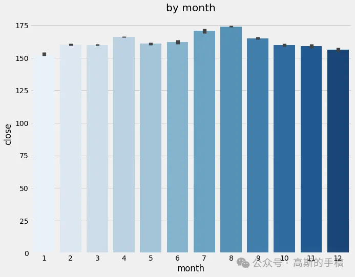
Create Our Model
train = create_features(train)
test = create_features(test)

FEATURES = ['dayofyear', 'hour', 'dayofweek', 'quarter', 'month', 'year']
TARGET = 'close'

X_train = train[FEATURES]
y_train = train[TARGET]

X_test = test[FEATURES]
y_test = test[TARGET]
reg = xgb.XGBRegressor(base_score=mean, n_estimators=1000, early_stopping_rounds=1000, objective='reg:squarederror', max_depth=3, learning_rate=0.1)
reg.fit(X_train, y_train, eval_set=[(X_train, y_train), (X_test, y_test)], verbose=100)[0] validation_0-rmse:13.77227 validation_1-rmse:19.10013
[100] validation_0-rmse:2.21008 validation_1-rmse:28.93545
[200] validation_0-rmse:1.69919 validation_1-rmse:29.13252
[300] validation_0-rmse:1.53636 validation_1-rmse:29.19358
[400] validation_0-rmse:1.43590 validation_1-rmse:29.21800
[500] validation_0-rmse:1.36775 validation_1-rmse:29.23179
[600] validation_0-rmse:1.30781 validation_1-rmse:29.24437
[700] validation_0-rmse:1.26732 validation_1-rmse:29.24926
[800] validation_0-rmse:1.23259 validation_1-rmse:29.25145
[900] validation_0-rmse:1.20048 validation_1-rmse:29.25439
[999] validation_0-rmse:1.17463 validation_1-rmse:29.25731XGBRegressor(base_score=162.3033402402023, booster='gbtree', callbacks=None,
colsample_bylevel=1, colsample_bynode=1, colsample_bytree=1,
early_stopping_rounds=1000, enable_categorical=False,
eval_metric=None, gamma=0, gpu_id=-1, grow_policy='depthwise',
importance_type=None, interaction_constraints='',
learning_rate=0.1, max_bin=256, max_cat_to_onehot=4,
max_delta_step=0, max_depth=3, max_leaves=0, min_child_weight=1,
missing=nan, monotone_constraints='()', n_estimators=1000,
n_jobs=0, num_parallel_tree=1, predictor='auto', random_state=0,
reg_alpha=0, reg_lambda=1, ...)Forecast on Test
test['prediction'] = reg.predict(X_test)
test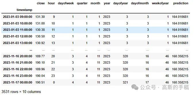
test['prediction'].mean()161.7173import matplotlib.pyplot as plt
plt.figure(figsize=(20, 6))
plt.plot(test['close'], label='Actual', color='blue')
plt.plot(test['prediction'], label='Predicted', color='red')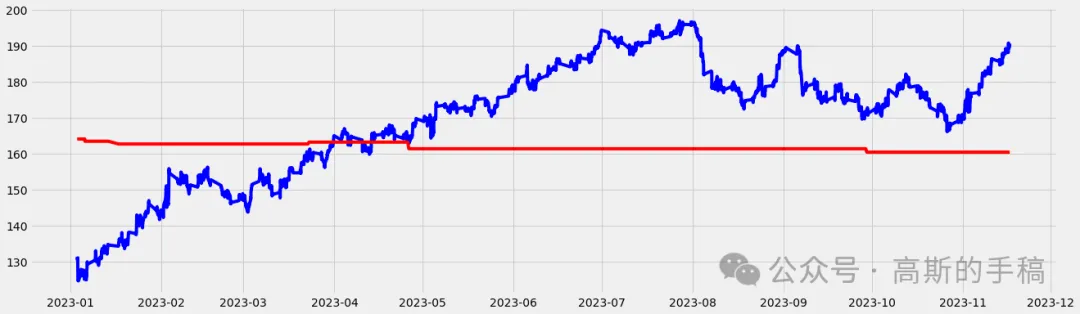
df = pd.merge(df, test, on="time")df.tail()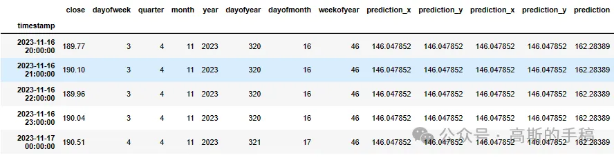
ax = df[['close']].plot(figsize=(15, 5))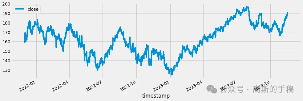
df['prediction'].plot(ax=ax, style='.')
plt.legend(['Truth Data', 'Predictions'])
ax.set_title('Raw Data and Prediction')
plt.show()
ax = df.loc[(df.index > '04-01-2018') & (df.index < '04-08-2018')]['PJME_MW'] \
.plot(figsize=(15, 5), title='Week Of Data')
df.loc[(df.index > '04-01-2018') & (df.index < '04-08-2018')]['prediction'] \
.plot(style='.')
plt.legend(['Truth Data','Prediction'])
plt.show()Score (RMSE)
score = np.sqrt(mean_squared_error(test['close'], test['prediction']))
print(f'RMSE Score on Test set: {score:0.2f}')
RMSE Score on Test set: 28.61
Content generated by AI

Edit / Fan Ruqiang
Review / Fan Ruqiang
Verification / Fan Ruqiang
Click below
Follow us