Translated by: Lin Likun
Proofread by: zrx


This article is about 6700 words long and is recommended for a 10-minute read.
This article discusses the performance analysis and optimization of PyTorch models.

Photo by Torsten Dederichs, uploaded to Unsplash
Training deep learning models, especially large ones, can be an expensive endeavor. Performance optimization is one of our main methods for reducing costs. Performance optimization is an iterative process in which we continuously seek opportunities to improve application performance and take advantage of them. In previous articles, we have emphasized the importance of using the right tools for analysis. The choice of tools may depend on various factors, including the type of training accelerator (such as GPU, HPU, or others) and the training framework.
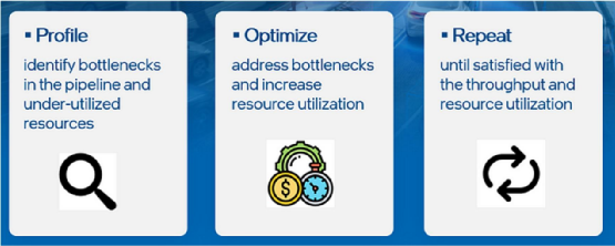
Performance optimization process (from the author)
This article focuses on training using PyTorch on GPUs. Specifically, we will focus on PyTorch’s built-in performance analyzer, the PyTorch Profiler, and one of the ways to view its results, which is the PyTorch Profiler TensorBoard plugin.
This article is not intended to replace the official PyTorch documentation on the PyTorch Profiler or on analyzing profiler results with the TensorBoard plugin. Our goal is to demonstrate how to use these tools in daily development processes. In fact, if you have not read the official documentation, we recommend that you do so before reading this article.
For some time, I have been interested in the TensorBoard plugin tutorial. The tutorial introduces a classification model based on the Resnet architecture, which is trained on the popular CIFAR10 dataset. Next, it will demonstrate how to use the PyTorch Profiler and TensorBoard plugin to identify and fix bottlenecks in the data loader. Performance bottlenecks in the input data pipeline are not uncommon, and we have discussed them in detail in some of our previous articles. What is surprising in the tutorial is the final (optimized) results (as of the time of writing this article), which we will paste below:
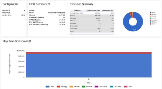
Optimized performance (excerpt from the PyTorch website)
If you look closely, you will notice that the optimized GPU utilization is 40.46%. Now, there is no way to sugarcoat this: these results are absolutely dismal and should keep you up at night. As we have explained in the past, GPUs are the most expensive resources in a training machine, and our goal should be to maximize their utilization. A utilization of 40.46% typically represents a significant opportunity for training acceleration and cost savings. Of course, we can do better! In this blog post, we will try to do better. First, we will attempt to reproduce the results presented in the official tutorial and see if we can further improve training performance using the same tools.
Simple Example
The code block below contains the training loop defined in the TensorBoard plugin tutorial, with two minor modifications:
We used a fake dataset that has the same attributes and behavior as the CIFAR10 dataset used in the tutorial. The motivation for this change can be found here.
We set the warmup flag to 3 and the repeat flag to 1 at initialization. We found that a slight increase in the number of warmup steps improved the stability of the results.
import numpy as np
import torch
import torch.nn
import torch.optim
import torch.profiler
import torch.utils.data
import torchvision.datasets
import torchvision.models
import torchvision.transforms as T
from torchvision.datasets.vision import VisionDataset
from PIL import Image


class FakeCIFAR(VisionDataset):
    def __init__(self, transform):
        super().__init__(root=None, transform=transform)
        self.data = np.random.randint(low=0, high=256, size=(1_000_032, 323), dtype=np.uint8)
        self.targets = np.random.randint(low=0, high=10, size=(10000), dtype=np.uint8).tolist()

    def __getitem__(self, index):
        img, target = self.data[index], self.targets[index]
        img = Image.fromarray(img)
        if self.transform is not None:
            img = self.transform(img)
        return img, target

    def __len__(self) -> int:
        return len(self.data)

transform = T.Compose([
    T.Resize(224),
    T.ToTensor(),
    T.Normalize((0.5, 0.5, 0.5), (0.5, 0.5, 0.5))
])

train_set = FakeCIFAR(transform=transform)
train_loader = torch.utils.data.DataLoader(train_set, batch_size=32, shuffle=True)

device = torch.device("cuda:0")
model = torchvision.models.resnet18(weights='IMAGENET1K_V1').cuda(device)
criterion = torch.nn.CrossEntropyLoss().cuda(device)
optimizer = torch.optim.SGD(model.parameters(), lr=0.001, momentum=0.9)
model.train()

# train step
def train(data):
    inputs, labels = data[0].to(device=device), data[1].to(device=device)
    outputs = model(inputs)
    loss = criterion(outputs, labels)
    optimizer.zero_grad()
    loss.backward()
    optimizer.step()

# training loop wrapped with profiler object
with torch.profiler.profile(
    schedule=torch.profiler.schedule(wait=1, warmup=4, active=3, repeat=1),
    on_trace_ready=torch.profiler.tensorboard_trace_handler('./log/resnet18'),
    record_shapes=True,
    profile_memory=True,
    with_stack=True
) as prof:
    for step, batch_data in enumerate(train_loader):
        if step >= (1 + 4 + 3) * 1:
            break
        train(batch_data)
        prof.step()  # Need to call this at the end of each step
The GPU used in the tutorial is Tesla V100-DGXS-32GB. In this article, we attempt to reproduce and improve the performance results from the tutorial using an Amazon EC2 p3.2xlarge instance that includes a Tesla V100-SXM2-16GB GPU. While they share the same architecture, there are some differences between these two GPUs. You can learn about these differences here. We ran the training script using the AWS PyTorch 2.0 Docker image. The performance results of the training script are displayed on the preview page of the TensorBoard viewer, as shown in the figure below:
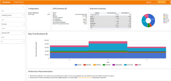
Baseline performance results shown in the TensorBoard Profiler overview tab (author’s screenshot)
First, we noticed that, contrary to the tutorial, our overview page (torrent-tb-profiler version 0.4.1) combined three steps into one. Therefore, the average time for the entire step is 80 milliseconds, rather than the 240 milliseconds reported. This can be clearly seen from the tracing tab (which, in our experience, almost always provides a more accurate report), where each step took about 80 milliseconds.
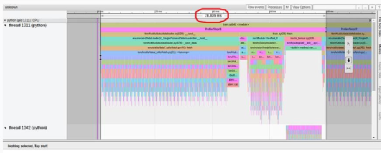
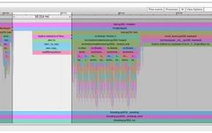
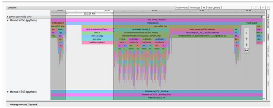
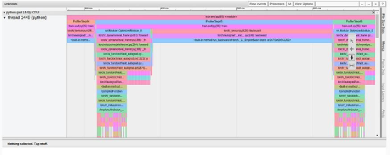
Baseline performance results shown in the TensorBoard Profiler tracing view tab (author’s screenshot)
Please note that our starting point (31.65% GPU utilization and 80 milliseconds step time) differs from the starting point in the tutorial (23.54% and 132 milliseconds, respectively). This may be due to differences in the training environment, including GPU type and PyTorch version. We also noted that the baseline results from the tutorial explicitly diagnosed performance issues as bottlenecks in the data loader, whereas our results did not. We often find that data loading bottlenecks masquerade as high percentages of “CPU execution” or “others” in the overview tab.
Optimization #1: Multi-process Data Loading
First, let’s use multi-process data loading as described in the tutorial. Given that the Amazon EC2 p3.2xlarge instance has 8 vCPUs, we will set the number of data loader workers to 8 for maximum performance:
train_loader = torch.utils.data.DataLoader(train_set, batch_size=32, shuffle=True, num_workers=8)
The optimization results are as follows:
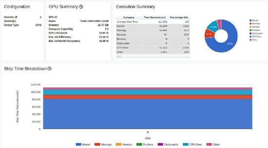
Results from multi-process data loading in the TensorBoard Profiler overview tab (author’s screenshot)
With just one line of code modified, GPU utilization increased by over 200% (from 31.65% to 72.81%), and training step time was reduced by more than half (from 80 milliseconds to 37 milliseconds).
The optimization process in the tutorial ends here. While our GPU utilization (72.81%) is significantly higher than the results in the tutorial (40.46%), I have no doubt that you, like us, would still find these results unsatisfactory.
Author’s Comment:Imagine how much could be saved globally if PyTorch applied multi-process data loading by default when training on GPUs? Admittedly, there may be some unnecessary side effects when using multi-processing. However, there must be some form of automatic detection algorithm that can run to exclude potential problem scenarios and apply this optimization accordingly.
Optimization #2: Pin Memory
If we analyze the tracing view from the last experiment, we will find that a significant amount of time (10 milliseconds out of 37 milliseconds) is still spent loading training data onto the GPU.
Results from multi-process data loading in the tracing view tab (author’s screenshot)
To address this issue, we will apply another optimization method recommended by PyTorch to simplify the data input flow, which is pinning memory. Using pinned memory can speed up the host-to-GPU data copy, and more importantly, we can make them asynchronous. This means we can prepare the next training batch in the GPU while training on the current batch. Note that while asynchronous processing can optimize performance, it may reduce the accuracy of time measurements. In this blog post, we will continue to use the measurement results reported by the PyTorch Profiler. For more details and potential side effects of pinning memory, as well as instructions on how to measure accurately, please refer to the PyTorch documentation.
This optimization requires modifying two lines of code. First, we set pin_memory to True in the data loader.
train_loader = torch.utils.data.DataLoader(train_set, batch_size=32, shuffle=True, num_workers=8, pin_memory=True)
Then, we modify the memory transfer from host to device (in the training function) to be non-blocking:
inputs, labels = data[0].to(device=device, non_blocking=True),
                           data[1].to(device=device, non_blocking=True)
|
Results after pinning memory optimization are shown below:
|

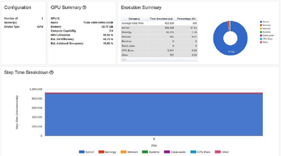
Results from pin memory optimization in the TensorBoard Profiler overview tab (author’s screenshot)
Now, our GPU utilization has reached 92.37%, and step time has further decreased. But we can still do better. Note that despite the optimizations, the performance report still shows that we are spending a significant amount of time copying data to the GPU. We will revisit this issue again in step 4 below.
Optimization #3: Increase Batch Size
In the next optimization step, we will focus on the “memory view” from the last experiment:
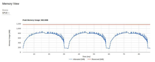
TensorBoard Profiler memory view (screenshot by the author)
The chart shows that in 16 GB of GPU memory, our peak utilization is less than 1 GB. This is an extreme example of underutilization of resources, which usually (but not always) indicates an opportunity to improve performance. One way to control memory utilization is to increase the batch size. In the figure below, we show the performance results when the batch size is increased to 512 (memory utilization increased to 11.3 GB).

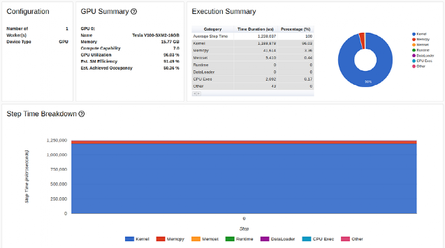
Results from increasing batch size in the TensorBoard Profiler overview tab (author’s screenshot)
While there is not much change in GPU utilization, our training speed improved significantly, from 1200 samples per second (46 milliseconds for a batch size of 32) to 1584 samples per second (324 milliseconds for a batch size of 512).
Note: In contrast to our previous optimizations, increasing the batch size may affect the behavior of the training application. Different models may respond differently to changes in batch size. Some models may only require minor adjustments to the optimization settings. For others, adjusting to a large batch size may be more challenging, or even impossible. Please refer to the previous article for some of the challenges faced with large batch training.
Optimization #4: Reduce Host-to-Device Copies
You may have noticed that in our previous results, the large red block in the pie chart represents the host-to-device data copy. The most straightforward way to address this bottleneck is to see if we can reduce the amount of data per batch. Note that in the case of image inputs, we convert the data type from 8-bit unsigned integers to 32-bit floats and perform normalization before the data copy. In the code block below, we suggest modifying the input data stream to delay the data type conversion and normalization until after the data enters the GPU:
# maintain the image input as an 8-bit uint8 tensor
transform = T.Compose([
    T.Resize(224),
    T.PILToTensor()
])
train_set = FakeCIFAR(transform=transform)
train_loader = torch.utils.data.DataLoader(train_set, batch_size=1024, shuffle=True, num_workers=8, pin_memory=True)

device = torch.device("cuda:0")
model = torch.compile(torchvision.models.resnet18(weights='IMAGENET1K_V1').cuda(device), fullgraph=True)
criterion = torch.nn.CrossEntropyLoss().cuda(device)
optimizer = torch.optim.SGD(model.parameters(), lr=0.001, momentum=0.9)
model.train()

# train step
def train(data):
    inputs, labels = data[0].to(device=device, non_blocking=True),
                           data[1].to(device=device, non_blocking=True)
    # convert to float32 and normalize
    inputs = (inputs.to(torch.float32) / 255. - 0.5) / 0.5
    outputs = model(inputs)
    loss = criterion(outputs, labels)
    optimizer.zero_grad()
    loss.backward()
    optimizer.step()
Due to this change, the amount of data copied from CPU to GPU was reduced by a factor of 4, and the unsightly red block has nearly disappeared:
Results from reducing CPU-to-GPU copies in the TensorBoard Profiler overview tab (author’s screenshot)
Now, our GPU utilization has reached a new high of 97.51% (!!), and the training speed reached 1670 samples per second! Let’s see what else we can do.
Optimization #5: Set Gradients to None
At this stage, we seem to have fully utilized the GPU, but that doesn’t mean we can’t use it more efficiently. There is a popular optimization method said to reduce memory operations in the GPU, which is to set the model parameter gradients to “none” instead of zero at each training step. Please refer to the PyTorch documentation for more details on this optimization. To implement this optimization, simply set the set_to_none parameter in the optimizer.zero_grad call to True:
optimizer.zero_grad(set_to_none=True)
In our case, this optimization did not meaningfully improve our performance.
Optimization #6: Automatic Mixed Precision
The GPU kernel view shows the active time of GPU kernels, which is a useful resource for improving GPU utilization:
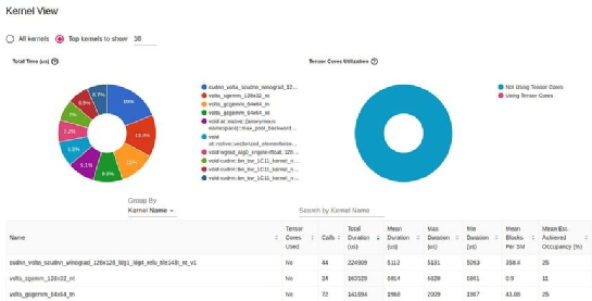
Kernel view in TensorBoard Profiler (captured by the author)
One of the most striking details in this report is the lack of usage of GPU Tensor Cores. Tensor Cores, which are dedicated processing units for matrix multiplication, can significantly boost the performance of AI applications on newer GPU architectures. The lack of Tensor Core usage indicates that there may be a significant optimization opportunity.
Since Tensor Cores are designed specifically for mixed precision computation, one direct way to improve the utilization is to modify our model to use automatic mixed precision (AMP). In AMP mode, parts of the model are automatically converted to lower precision 16-bit floats and run on GPU tensor cores.
Importantly, please note that full implementation of AMP may require gradient scaling, which our demonstration does not include. Please be sure to check the relevant documentation on mixed precision training before making adjustments.
The code block below demonstrates the modifications made to the training step to enable AMP.
def train(data):
    inputs, labels = data[0].to(device=device, non_blocking=True),
                           data[1].to(device=device, non_blocking=True)
    inputs = (inputs.to(torch.float32) / 255. - 0.5) / 0.5
    with torch.autocast(device_type='cuda', dtype=torch.float16):
        outputs = model(inputs)
        loss = criterion(outputs, labels)
    # Note - torch.cuda.amp.GradScaler() may be required
    optimizer.zero_grad(set_to_none=True)
    loss.backward()
    optimizer.step()
The following figure shows the impact on the utilization of “Tensor Cores”. While it continues to indicate that there is still room for further improvement, with just one line of code,
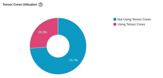
Utilization jumped from 0% to 26.3%.
Tensor Core utilization with AMP optimization in TensorBoard Profiler kernel view (author’s screenshot)
In addition to improving Tensor Core utilization, using AMP can also reduce GPU memory utilization, freeing up more space for increasing batch size. The figure below shows the training performance results after AMP optimization, with batch size set to 1024:
AMP optimization results in the TensorBoard Profiler overview tab (author’s screenshot)
While GPU utilization slightly decreased, our key throughput metric further improved by nearly 50%, from 1670 samples per second to 2477 samples per second. Our optimizations are working!
Note: Reducing the precision of some models may significantly affect their convergence. As with increasing batch size (see above), the impact of using mixed precision varies by model. In some cases, using AMP may barely change performance. In others, you may need to invest more effort to adjust the autoscaler. There are also instances where you may need to explicitly set the precision type for different parts of the model (i.e., manual mixed precision).
For more details on using mixed precision as a memory optimization method, please refer to our previous related blog posts.
Optimization #7: Train in Graph Mode
The final optimization we will apply is model compilation. Unlike PyTorch’s default eager execution mode (where every PyTorch operation runs “eagerly”), the compile API converts your model into an intermediate computation graph and compiles it into lower-level compute kernels in a way that is optimal for the underlying training accelerator. For more information on model compilation in PyTorch 2, please refer to our previously published articles.
The code block below demonstrates the changes required to apply model compilation:
model = torchvision.models.resnet18(weights='IMAGENET1K_V1').cuda(device)
model = torch.compile(model)
The results of model compilation optimization are shown below:
Model compilation results in the TensorBoard Profiler overview tab (author’s screenshot)
Model compilation further increased our throughput to 3268 samples per second, up from 2477 samples per second in previous experiments, representing a 32% performance increase (!!).
The way model compilation changes the training step is very evident in the different views of the TensorBoard plugin. For example, the “kernel view” shows the use of new (fused) GPU kernels, while the “tracing view” (as shown in the figure below) displays a pattern that is completely different from what we saw before.
TensorBoard Profiler tracing view tab model compilation results (author’s screenshot)
Temporary Results
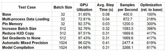
We summarize a series of optimization results in the table below.
Performance Results Summary (author)
By using the PyTorch Profiler and TensorBoard plugin for iterative analysis and optimization, we improved performance by 817%!
Are we done? Absolutely not! Each optimization we implement uncovers new potential performance improvement opportunities. These opportunities come in the form of resource release (for example, switching to mixed precision allowed us to increase the batch size) or the emergence of newly discovered performance bottlenecks (for example, our final optimization uncovered a bottleneck in host-to-device data transfer). Additionally, there are many other well-known forms of optimization that we did not attempt in this article (see here and here). Finally, new optimization libraries (such as the model compilation feature we demonstrated in step 7) are constantly being released to further achieve our performance enhancement goals. As we emphasized in the introduction, to fully leverage these opportunities, performance optimization must be an iterative and ongoing part of the development workflow.
Conclusion
In this article, we demonstrated the tremendous potential for simple model performance optimization. While there are other performance analyzers available, each with its pros and cons, we chose the PyTorch Profiler and TensorBoard plugin for their ease of integration.
We must emphasize that the path to successful optimization can vary greatly depending on the specifics of the training project, including model structure and training environment. In practice, achieving goals may be more difficult than the examples we presented here. Some techniques we introduced may have little impact on performance or may even degrade it. We also noted that the precise optimization methods we chose and the order in which we applied them were somewhat arbitrary. We strongly recommend that you develop your own tools and techniques tailored to the specific details of your project to achieve your optimization goals.
Performance optimization for machine learning workloads is sometimes seen as secondary, non-essential, and tedious. I hope we have successfully convinced you that the potential to save development time and costs is worth your investment in performance analysis and optimization. And hey, you might even find it fun 🙂
What’s Next?
This is just the tip of the iceberg. Performance optimization involves much more than this. In the sequel to this article, we will delve into a very common performance issue in PyTorch models: performing too much computation on the CPU rather than the GPU, often without the developers’ knowledge. We also encourage you to check out our other articles published on Medium, many of which cover different aspects of performance optimization for machine learning workloads.
Original Title:
PyTorch Model Performance Analysis and Optimization
Original Link:
PyTorch Model Performance Analysis and Optimization | by Chaim Rand | Towards Data Science
Lin Likun, an undergraduate in Computational Mathematics at City University of Hong Kong, is a data science enthusiast with a particular interest in the intersection of mathematics and computer science. His interests include playing badminton and exploring some quirky learning tools. He hopes to share higher quality articles and more valuable content with readers through his efforts, making their learning experience in data science smoother!
Translation Team Recruitment Information
Job Description: Requires a meticulous heart to translate selected foreign articles into fluent Chinese. If you are an overseas student in data science/statistics/computer-related fields, or working overseas in related jobs, or confident in your language skills, you are welcome to join the translation team.
What You Can Get: Regular translation training to improve volunteers’ translation skills and enhance their understanding of the cutting edge of data science. Overseas friends can stay connected with the development of technology applications in China. The background of THU Data Team provides good development opportunities for volunteers.
Other Benefits: Data scientists from renowned companies, students from prestigious universities such as Peking University and Tsinghua University, and overseas students will all become your partners in the translation team.
Click the “Read Original” at the end to join the Data Team~
Reprint Notice
If you need to reprint, please indicate the author and source prominently at the beginning (reprinted from: Data Team ID: DatapiTHU), and place a prominent QR code of the Data Team at the end of the article. For articles with original markings, please send [article name – waiting for authorization public account name and ID] to the contact email to apply for whitelist authorization and edit as required.
After publishing, please provide the link to the contact email (see below). Unauthorized reprints and adaptations will be pursued legally.
Click“Read Original” to embrace the organization