

Source: DeepHub IMBA


This article is about 6400 words long and is recommended for a 12-minute read.
In this article, we will demonstrate the use of new features in PyTorch 2.0 and highlight some issues you might encounter when using it.
It has been some time since the release of PyTorch 2.0. Have you started using it? PyTorch 2.0 significantly improves training and inference speed by introducing torch.compile. Unlike eager mode, the compile API converts the model into an intermediate computation graph (FX graph) and then compiles it into low-level computation kernels, thus enhancing execution speed.

For PyTorch 2.0, what you might see is:
“Just wrap them with torch.compile to speed up execution”
However, many factors can interfere with the compilation of the computation graph and/or achieving the desired performance improvements. Therefore, adjusting the model and achieving optimal performance may require redesigning the project or modifying some coding habits.
In this article, we will demonstrate the use of this new feature and discuss some potential issues you might encounter when using it. We will share several examples of problems encountered when tweaking the torch.compile API. These examples are not exhaustive, and you may encounter issues not mentioned here in practical applications, especially since torch.compile is still under active development and has room for improvement.
Many innovative technologies are behind Torch compilation, including TorchDynamo, FX Graph, TorchInductor, Triton, etc. We will not delve into the different components in this article; if you are interested, you can check the PyTorch documentation, which provides detailed information.
Two Unimportant Comparisons Between TensorFlow and PyTorch
1. In the past, there were clear distinctions between PyTorch and TensorFlow. PyTorch used eager execution mode, while TensorFlow used graph mode, with both evolving separately. However, TensorFlow 2 later introduced eager execution as the default execution mode, making TensorFlow somewhat resemble PyTorch. Now, PyTorch has also introduced its own graph mode solution, making it somewhat similar to TensorFlow. The competition between TensorFlow and PyTorch continues, but the differences between the two are gradually diminishing.
2. AI development is a trendy industry. However, popular AI models, model architectures, learning algorithms, training frameworks, etc., evolve over time. In terms of papers, most of the models we dealt with a few years ago were written in TensorFlow. However, many people often complained that the high-level model.fit API limited their development flexibility and that the graph mode hindered their debugging. Consequently, many turned to PyTorch, claiming, “PyTorch allows you to build models in any way you want and debug easily.” However, more flexible custom operations lead to increased complexity in development, and the emergence of high-level APIs like PyTorch Lightning replicates the features of model.fit, leading to further claims of needing to adapt to PyTorch Lightning and accelerate their training with torch.compile. Achieving both flexibility and simplicity simultaneously is impossible.
Main Content Begins
Now let’s introduce a collection of tips on how to use the PyTorch 2 compilation API and some potential issues you may face. Adapting models to PyTorch’s graph mode may require considerable effort. We hope this article helps you better assess this effort and decide on the best way to take this step.
Installing PyTorch 2
According to the PyTorch installation documentation, installing PyTorch 2 seems no different from installing any other version of PyTorch. However, in practice, you may encounter some issues. First, PyTorch 2.0 (as of this article) requires Python 3.8 or higher. Additionally, PyTorch 2 includes package dependencies that were not present in previous versions (most notably PyTorch-triton, which I don’t even know what it is, haha), and you should be aware that this may introduce new conflicts.
So if you are familiar with Docker, it is recommended to use containers directly, which will simplify things a lot.
PyTorch 2 Compatibility
One of the advantages of PyTorch 2 is that it is fully backward compatible, so even if we do not use torch.compile, we can still use PyTorch 2.0 and benefit from other new features and enhancements. At most, we will not enjoy speed improvements, but there will be no compatibility issues. However, if you want to further enhance speed, please continue reading.
Simple Example
Let’s start with a simple example of an image classification model. In the code block below, we use the timm Python package (version 0.6.12) to build a basic Vision Transformer (ViT) model and train it for 500 steps (not epochs) on a fake dataset. Here, we define the use_compile flag to control whether to execute model compilation (torch.compile), and use_amp to control whether to use automatic mixed precision (AMP) or full precision (FP) execution.
 import time, os
import torch
from torch.utils.data import Dataset
from timm.models.vision_transformer import VisionTransformer

use_amp = True  # toggle to enable/disable amp
use_compile = True  # toggle to use eager/graph execution mode

# use a fake dataset (random data)
class FakeDataset(Dataset):
    def __len__(self):
        return 1000000

    def __getitem__(self, index):
        rand_image = torch.randn([3, 224, 224], dtype=torch.float32)
        label = torch.tensor(data=[index % 1000], dtype=torch.int64)
        return rand_image, label

def train():
    device = torch.cuda.current_device()
    dataset = FakeDataset()
    batch_size = 64

    # define an image classification model with a ViT backbone
    model = VisionTransformer()
    if use_compile:
        model = torch.compile(model)
    model.to(device)
    optimizer = torch.optim.Adam(model.parameters())
    data_loader = torch.utils.data.DataLoader(dataset,
                                               batch_size=batch_size, num_workers=4)
    loss_function = torch.nn.CrossEntropyLoss()
    t0 = time.perf_counter()
    summ = 0
    count = 0
    for idx, (inputs, target) in enumerate(data_loader, start=1):
        inputs = inputs.to(device)
        targets = torch.squeeze(target.to(device), -1)
        optimizer.zero_grad()
        with torch.cuda.amp.autocast(
                enabled=use_amp,
                dtype=torch.bfloat16):
            outputs = model(inputs)
            loss = loss_function(outputs, targets)
        loss.backward()
        optimizer.step()
        batch_time = time.perf_counter() - t0
        if idx > 10:  # skip first few steps
            summ += batch_time
            count += 1
        t0 = time.perf_counter()
        if idx > 500:
            break
    print(f'average step time: {summ/count}')

if __name__ == '__main__':
    train()
The performance results are recorded in the table below. These results can vary significantly depending on the environment, so they are for reference only.
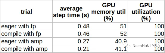
As we can see, using AMP (28.6%) yields significantly better performance improvements from model compilation compared to using FP (4.5%). This is a well-known difference. If you have not yet trained using AMP, the improvement in training speed comes from transitioning from FP to AMP, so I recommend starting with AMP. Additionally, the performance improvement comes with a very slight increase in GPU memory utilization.
When scaling to multiple GPUs, the performance comparisons may change due to the way distributed training is implemented on the compiled graph. For specific details, refer to the official documentation.
Advanced Options
The compile API includes many options for controlling graph creation, allowing for fine-tuning of compilation for specific models and possibly further improving performance. The code block below introduces the official function:
def compile(model: Optional[Callable] = None, *,
             fullgraph: builtins.bool = False,
             dynamic: builtins.bool = False,
             backend: Union[str, Callable] = "inductor",
             mode: Union[str, None] = None,
             options: Optional[Dict[str, Union[str, builtins.int, builtins.bool]]] = None,
             disable: builtins.bool = False) -> Callable:
    """
    Optimizes given model/function using TorchDynamo and specified backend.
    Args:
        model (Callable): Module/function to optimize
        fullgraph (bool): Whether it is ok to break model into several subgraphs
        dynamic (bool): Use dynamic shape tracing
        backend (str or Callable): backend to be used
        mode (str): Can be either "default", "reduce-overhead" or "max-autotune"
        options (dict): A dictionary of options to pass to the backend.
        disable (bool): Turn torch.compile() into a no-op for testing
    """
The mode compilation mode: allows you to choose between minimizing the overhead of compilation (“reduce-overhead”) and maximizing potential performance gains (“max-autotune”).
The table below compares the results of compiling the aforementioned ViT model under different compilation modes.
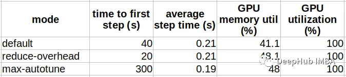
As we can see, the behavior of the compilation modes is quite similar to their names; “reduce-overhead” reduces compilation time at the cost of additional memory utilization, while “max-autotune” achieves optimal performance at the expense of high compilation time overhead.
The backend compiler backend: the API uses which backend to convert the intermediate representation (IR) computation graph (FX graph) into low-level kernel operations. This option is useful for debugging graph compilation issues and gaining a better understanding of the internals of torch.compile. In most cases, the default Inductor backend seems to provide the best training performance results. There are many backends available, and we can check them with the following command:
from torch import _dynamo
print(_dynamo.list_backends())
We tested using the nvprims-nvfuser backend, which achieved a 13% performance improvement over eager mode (compared to a 28.6% performance improvement with the default backend). The specific differences can be found in the PyTorch documentation, which we won’t elaborate on here, as the documentation is comprehensive.
The fullgraph parameter forces a single graph: this parameter is very useful to ensure that no unwanted graph truncation occurs.
The dynamic shape: Currently, support for compiling models with dynamic shapes in 2.0 is somewhat limited. A common solution for compiling models with dynamic shapes is to recompile, which significantly increases overhead and greatly reduces training speed. If your model does include dynamic shapes, setting the dynamic flag to True will yield better performance, especially reducing the frequency of recompilation.
What are dynamic shapes? The simplest example is time series or varying text lengths; if sequences have different lengths without alignment, they are dynamic shapes.
Performance Analysis
The PyTorch Profiler is one of the key tools for analyzing the performance of PyTorch models, allowing for the evaluation and analysis of how graph compilation optimizes training steps. In the code block below, we generate TensorBoard results with the profiler to examine training performance:
out_path = os.path.join(os.environ.get('SM_MODEL_DIR','/tmp'),'profile')
from torch.profiler import profile, ProfilerActivity
with profile(
        activities=[ProfilerActivity.CPU, ProfilerActivity.CUDA],
        schedule=torch.profiler.schedule(
            wait=20,
            warmup=5,
            active=10,
            repeat=1),
        on_trace_ready=torch.profiler.tensorboard_trace_handler(
                                            dir_name=out_path)
) as p:
    for idx, (inputs, target) in enumerate(data_loader, start=1):
        inputs = inputs.to(device)
        targets = torch.squeeze(target.to(device), -1)
        optimizer.zero_grad()
        with torch.cuda.amp.autocast(
                enabled=use_amp,
                dtype=torch.bfloat16):
            outputs = model(inputs)
            loss = loss_function(outputs, targets)
        loss.backward()
        optimizer.step()
        p.step()
The following image is a screenshot from TensorBoard generated by the PyTorch Profiler. It provides detailed information on the kernels running on the GPU during the training steps of the compiled model experiments.
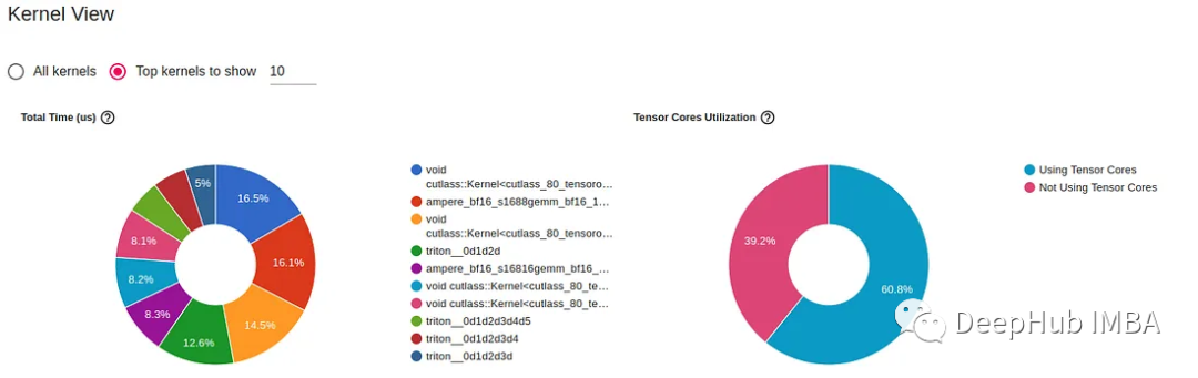
We can see that torch.compile has increased the utilization of GPU tensor cores (from 51% to 60%) and introduced GPU kernels developed using Triton.
Debugging Model Compilation Issues
torch.compile is currently in testing, and if you encounter issues, you may be lucky enough to receive an error message that you can search for a solution, or ask ChatGPT. However, if you are less fortunate, you will need to find the root of the problem yourself.
The main resource for resolving compilation issues is the TorchDynamo troubleshooting documentation, which includes a list of debugging tools and provides step-by-step guides for diagnosing errors. However, these tools and techniques currently seem more targeted at PyTorch developers rather than PyTorch users. They may help resolve underlying issues causing compilation problems, but there is a very high likelihood that they will not be helpful at all. So what should you do?
Here, we demonstrate a process for self-troubleshooting that can help resolve some issues.
Below is a simple distributed model that includes a call to torch.distributed.all_reduce. The model runs as expected in eager mode, but fails during graph compilation with an “attribute error” (torch.classes.c10d.ProcessGroup does not have a field with name ‘shape’). We need to raise the log level to INFO and then discover that the error occurs during the computation’s “step 3”, which is TorchInductor. Then we verify whether the compilation succeeds with the “eager” and “aot_eager” backends and finally create a minimal code example to reproduce the failure using PyTorch Minifier.
import os, logging
import torch
from torch import _dynamo

# enable debug prints
torch._dynamo.config.log_level = logging.INFO
torch._dynamo.config.verbose=True

# uncomment to run minifier
# torch._dynamo.config.repro_after="aot"

def build_model():
    import torch.nn as nn
    import torch.nn.functional as F

    class DumbNet(nn.Module):
        def __init__(self):
            super().__init__()
            self.conv1 = nn.Conv2d(3, 6, 5)
            self.pool = nn.MaxPool2d(2, 2)
            self.fc1 = nn.Linear(1176, 10)

        def forward(self, x):
            x = self.pool(F.relu(self.conv1(x)))
            x = torch.flatten(x, 1)
            with torch.no_grad():
                sum_vals = torch.sum(x, 0)
                # this is the problematic line of code
                torch.distributed.all_reduce(sum_vals)
            return x

    net = DumbNet()
    return net

def train():
    os.environ['MASTER_ADDR'] = os.environ.get('MASTER_ADDR', 'localhost')
    os.environ['MASTER_PORT'] = os.environ.get('MASTER_PORT', str(2222))
    torch.distributed.init_process_group('nccl', rank=0, world_size=1)
    torch.cuda.set_device(0)
    device = torch.cuda.current_device()

    model = build_model()
    model = torch.compile(model)
    # replace with this to verify that error is not in TorchDynamo
    # model = torch.compile(model, 'eager')
    # replace with this to verify that error is not in AOTAutograd
    # model = torch.compile(model, 'aot_eager')
    model.to(device)
    rand_image = torch.randn([4, 3, 32, 32], dtype=torch.float32).to(device)
    model(rand_image)

if __name__ == '__main__':
    train()
In this example, running the generated minifier_launcher.py script results in different attribute errors (e.g., Repro’ object has no attribute ‘_tensor_constant0’), which is not very helpful for our demonstration. We will temporarily ignore this, which also indicates that torch.compile is not yet perfect and has significant room for improvement. In other words, if you cannot resolve the issue, it might be better not to use it; at least “slow” is better than “not working,” right? (And the speed improvement is also limited)
Common Graph Truncation Issues
One of the advantages of PyTorch eager mode is the ability to interleave pure Pythonic code with PyTorch operations. However, this freedom is greatly restricted when using torch.compile. Pythonic operations can cause TorchDynamo to split the computation graph into multiple components, hindering the potential for performance enhancement. Our goal in code optimization is to minimize such graph truncation as much as possible. The simplest way is to compile the model with the fullgraph flag. This can prompt the removal of any code that causes graph truncation and also inform us how to best adapt to the development habits of PyTorch 2. However, to run distributed code, it must be set to False, as the current implementation requires graph splitting for communication between GPUs. We can also use torch._dynamo.explain to analyze graph truncation.
The following code block demonstrates a simple model that has four potential graph truncations in its forward pass. However, this usage pattern is not uncommon in typical PyTorch models.
import torch
from torch import _dynamo
import numpy as np

def build_model():
    import torch.nn as nn
    import torch.nn.functional as F

    class DumbNet(nn.Module):
        def __init__(self):
            super().__init__()
            self.conv1 = nn.Conv2d(3, 6, 5)
            self.pool = nn.MaxPool2d(2, 2)
            self.fc1 = nn.Linear(1176, 10)
            self.fc2 = nn.Linear(10, 10)
            self.fc3 = nn.Linear(10, 10)
            self.fc4 = nn.Linear(10, 10)
            self.d = {}

        def forward(self, x):
            x = self.pool(F.relu(self.conv1(x)))
            x = torch.flatten(x, 1)
            assert torch.all(x >= 0)  # graph break
            x = self.fc1(x)
            self.d['fc1-out'] = x.sum().item()  # graph break
            x = self.fc2(x)
            for k in np.arange(1):  # graph break
                x = self.fc3(x)
            print(x)  # graph break
            x = self.fc4(x)
            return x

    net = DumbNet()
    return net

def train():
    model = build_model()
    rand_image = torch.randn([4, 3, 32, 32], dtype=torch.float32)
    explanation = torch._dynamo.explain(model, rand_image)
    print(explanation)

if __name__ == '__main__':
    train()
Graph truncation does not cause compilation to fail (unless the fullgraph flag is set). Therefore, it is very likely that the model is being compiled and executed but actually contains multiple graph truncations, which will slow it down.
Training Issue Troubleshooting
Currently, successfully compiling a model with PyTorch 2 is considered an achievement worth celebrating, but it does not guarantee that training will succeed.
Low-level kernels running on GPUs may behave differently between eager and graph modes. Certain high-level operations may exhibit different behaviors. You may find that operations running in eager mode fail in graph mode (e.g., torch.argmin). You may also notice numerical differences in computations affecting training.
Debugging in graph mode is much more challenging than in eager mode. In eager mode, each line of code is executed independently, and we can place breakpoints at any point in the code to obtain the values of tensors. In graph mode, the model defined by the code undergoes multiple transformations before processing, and breakpoints may not be triggered.
Therefore, it is advisable to first use eager mode, and once the model runs successfully, apply torch.compile to each part separately, or generate graph truncations by inserting print statements and/or Tensor.numpy calls, which may successfully trigger breakpoints in the code. In other words, using torch.compile can take longer for development, so the trade-off between training and development speed depends on your own choices.
But don’t forget what we mentioned earlier: your model may not run correctly after adding torch.compile, which is another hidden cost.
Including the Loss Function in the Graph
By using the torch.compile call to wrap the PyTorch model (or function), you enable graph mode. However, the loss function is not part of the compile call and is not included in the graph generated. Thus, the loss function is a relatively small part of the training step, and running it in eager mode does not incur much overhead. However, if you have a computationally intensive loss function, it can also be included in the compiled computation graph to further enhance performance.
In the code below, we define a loss function for performing model distillation from a large ViT model (with 24 ViT blocks) to a smaller ViT model (with 12 ViT blocks).
import torch
from timm.models.vision_transformer import VisionTransformer

class ExpensiveLoss(torch.nn.Module):
    def __init__(self):
        super(ExpensiveLoss, self).__init__()
        self.expert_model = VisionTransformer(depth=24)
        if torch.cuda.is_available():
            self.expert_model.to(torch.cuda.current_device())
        self.mse_loss = torch.nn.MSELoss()

    def forward(self, input, outputs):
        expert_output = self.expert_model(input)
        return self.mse_loss(outputs, expert_output)
This is a loss function that is computationally more intensive than CrossEntropyLoss. Here are two methods to execute it faster:
1. The loss function is wrapped in the torch.compile call, as shown below:
loss_function = ExpensiveLoss()
compiled_loss = torch.compile(loss_function)
The disadvantage of this method is that the compiled graph of the loss function does not intersect with the compiled graph of the model, but its advantage is clear: it is simple.
2. Create a wrapper model that includes both the model and the loss, compile them together, and return the resulting loss as output.
import time, os
import torch
from torch.utils.data import Dataset
from torch import nn
from timm.models.vision_transformer import VisionTransformer

# use a fake dataset (random data)
class FakeDataset(Dataset):
    def __len__(self):
        return 1000000

    def __getitem__(self, index):
        rand_image = torch.randn([3, 224, 224], dtype=torch.float32)
        label = torch.tensor(data=[index % 1000], dtype=torch.int64)
        return rand_image, label

# create a wrapper model for the ViT model and loss
class SuperModel(torch.nn.Module):
    def __init__(self):
        super(SuperModel, self).__init__()
        self.model = VisionTransformer()
        self.expert_model = VisionTransformer(depth=24 if torch.cuda.is_available() else 2)
        self.mse_loss = torch.nn.MSELoss()

    def forward(self, inputs):
        outputs = self.model(inputs)
        with torch.no_grad():
            expert_output = self.expert_model(inputs)
        return self.mse_loss(outputs, expert_output)

# a loss that simply passes through the model output
class PassthroughLoss(nn.Module):
    def __call__(self, model_output):
        return model_output

def train():
    device = torch.cuda.current_device()
    dataset = FakeDataset()
    batch_size = 64

    # create and compile the model
    model = SuperModel()
    model = torch.compile(model)
    model.to(device)
    optimizer = torch.optim.Adam(model.parameters())
    data_loader = torch.utils.data.DataLoader(dataset,
                                               batch_size=batch_size, num_workers=4)
    loss_function = PassthroughLoss()
    t0 = time.perf_counter()
    summ = 0
    count = 0
    for idx, (inputs, target) in enumerate(data_loader, start=1):
        inputs = inputs.to(device)
        targets = torch.squeeze(target.to(device), -1)
        optimizer.zero_grad()
        with torch.cuda.amp.autocast(
                enabled=True,
                dtype=torch.bfloat16):
            outputs = model(inputs)
            loss = loss_function(outputs)
        loss.backward()
        optimizer.step()
        batch_time = time.perf_counter() - t0
        if idx > 10:  # skip first few steps
            summ += batch_time
            count += 1
        t0 = time.perf_counter()
        if idx > 500:
            break
    print(f'average step time: {summ/count}')

if __name__ == '__main__':
    train()
This method has the disadvantage that when running the model in inference mode, you need to extract the actual model from the wrapper model.
The performance improvement for both options is approximately 8%, indicating that compiling the loss is also an important part of optimization.
Dynamic Shapes
The official documentation also states that support for compiling models with dynamic shapes in torch.compile is limited. The compile API includes a dynamic parameter to signal to the compiler, but the extent to which this helps improve performance is questionable. If you are trying to compile and optimize dynamic graphs and are facing issues, it is better not to use torch.compile, as it can be quite troublesome.
Conclusion
PyTorch 2.0’s compilation mode has significant potential to improve training and inference speeds, potentially leading to substantial cost savings. However, the amount of work required to realize this potential can vary greatly. Many public models only require a single line of code modification, while others, especially those containing non-standard operations, dynamic shapes, and/or extensive interleaved Python code, may prove to be counterproductive or even impossible to implement. Nevertheless, starting to modify models now is a good choice, as torch.compile appears to be an important and ongoing feature for PyTorch 2.
Editor: Yu Tengkai
Proofreader: Lin Yilin