Introduction
The transformer is a framework that cannot be overlooked in the field of NLP and even deep learning as a whole. Most large language models (LLMs) are trained using it to generate models, so the transformer is a framework that every robot developer or artificial intelligence developer cannot bypass. This article will gradually unveil the veil of the transformer from the top down.
Overview of Transformer
The Transformer model comes from the paper ‘Attention Is All You Need’.(https://arxiv.org/abs/1706.03762)
In the paper, it was initially proposed to improve the efficiency of machine translation. It uses the Self-Attention mechanism and Position Encoding to replace RNNs. Later, it was found that Self-Attention performed very well and the Transformer model could also be used in other areas, leading to the subsequent BERT and GPT series.
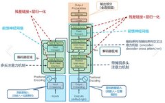
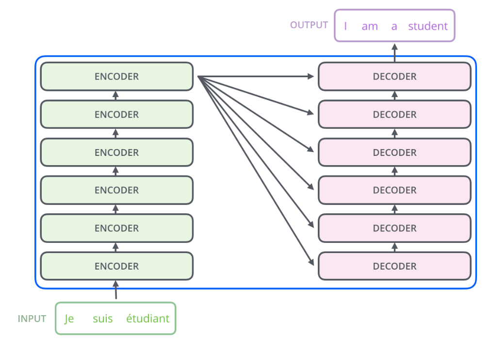
The transformer framework generally looks like the following diagram:
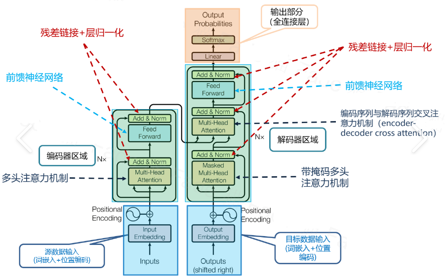
Overview of Transformer Model
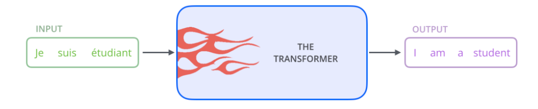
First, consider the model as a black box, as shown in the figure below. For machine translation, its input is a sentence in the source language (French), and its output is a sentence in the target language (English).
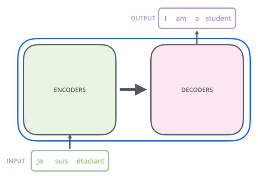
Opening the black box slightly, the Transformer (or any NMT system) can be divided into two parts: Encoder and Decoder, as shown in the figure below.
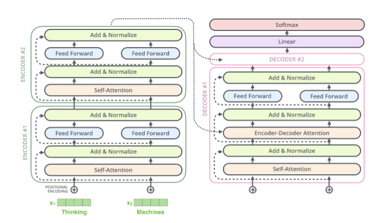
Expanding a bit further, the Encoder consists of many identical Encoder layers stacked together, and the Decoder is similar. As shown in the figure below.
The input to each Encoder is the output of the next layer of Encoder, and the input to the bottom layer Encoder is the original input (French sentence); the Decoder is similar, but the output of the last layer Encoder will be input to each layer of Decoder, which is required by the Attention mechanism.
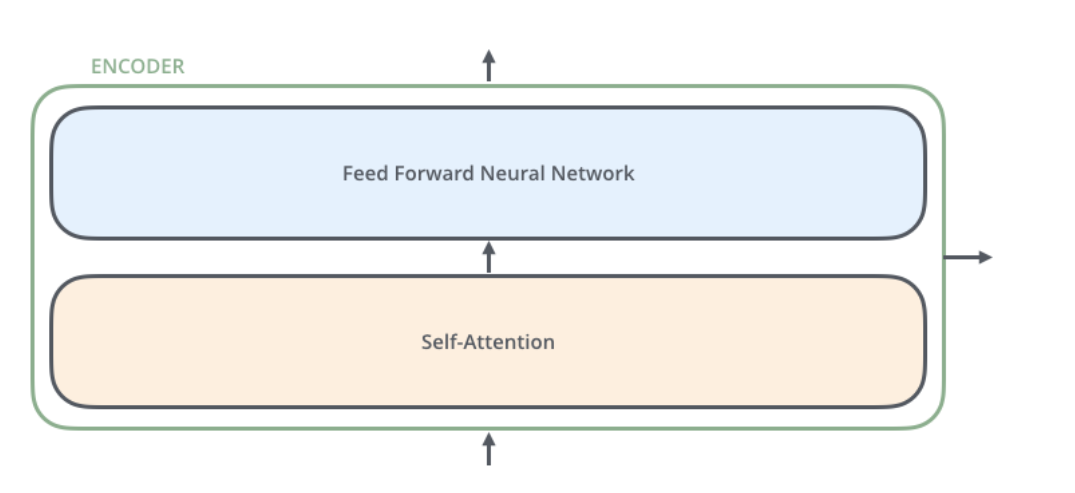
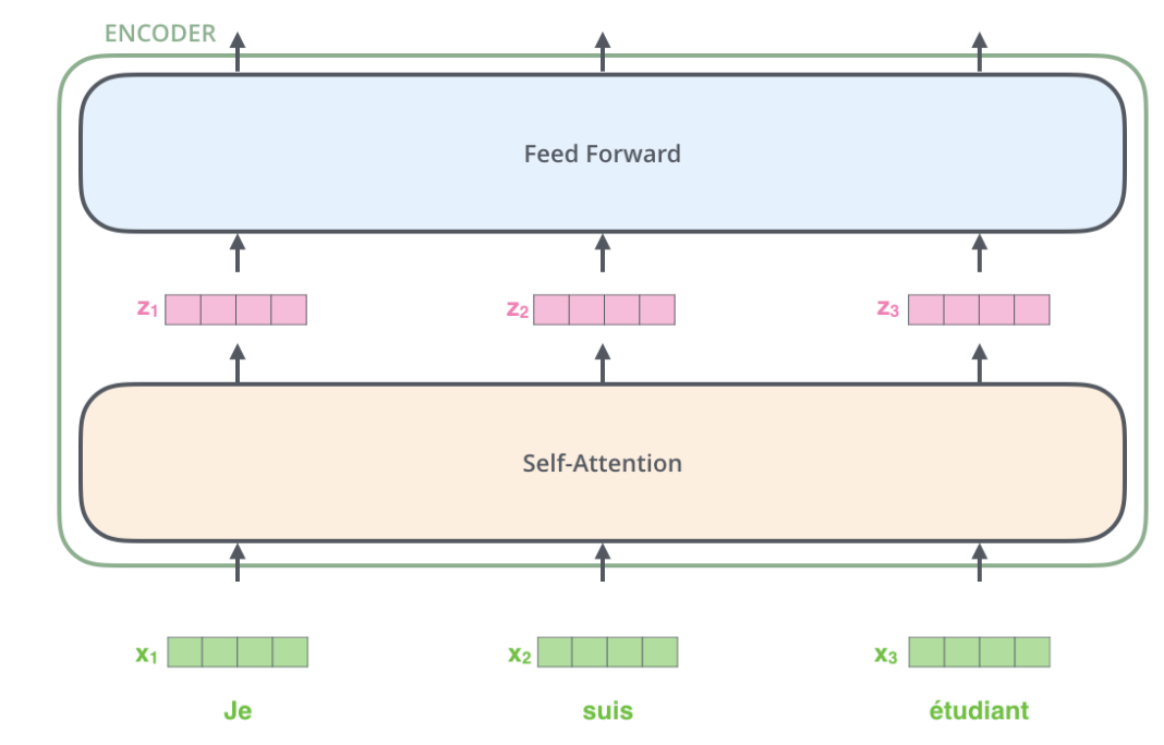
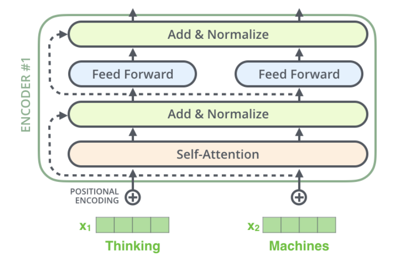
Each layer of the Encoder has the same structure, consisting of a Self-Attention layer and a feedforward network (fully connected network), as shown in the figure below.
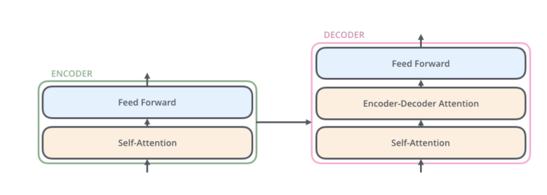
Each layer of the Decoder also has the same structure, but in addition to the Self-Attention layer and the fully connected layer, there is an additional Attention layer, which allows the Decoder to consider the outputs of the last layer of Encoder at all times during decoding. Its structure is shown in the figure below.
Transformer Process Flow
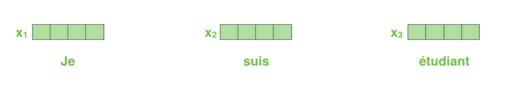
The flow of the transformer requires the addition of tensors. The input sentence needs to be transformed into a continuous dense vector through Embedding, as shown in the figure below.
The sequence after embedding will be input to the Encoder, first passing through the Self-Attention layer and then through the fully connected layer.
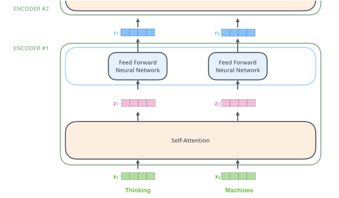
When calculating 𝑧𝑖, we need to rely on all inputs at all times 𝑥1,…,𝑥𝑛, which can be computed all at once using matrix operations. The computation of the fully connected network is completely independent; to compute the output at time i, it is sufficient to input 𝑧𝑖, so it can be easily parallelized. The figure below makes this clearer. In the figure, the Self-Attention layer is a large box, indicating that its input is all of 𝑥1,…,𝑥𝑛, and its output is 𝑧1,…,𝑧𝑛. The fully connected layer at each time is a box (but the parameters at different times are shared), indicating that computing 𝑟𝑖 only requires 𝑧𝑖. In addition, the outputs 𝑟1,…,𝑟𝑛 from the previous layer are directly input to the next layer.
Self-Attention Introduction
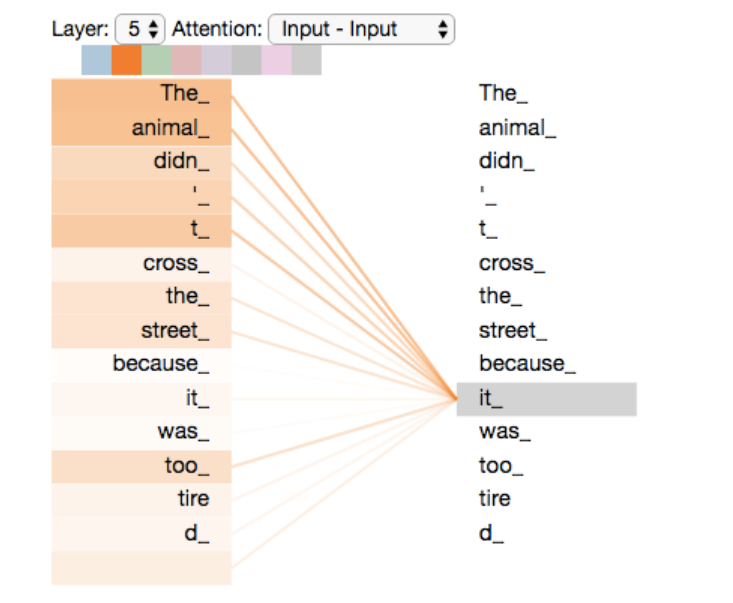
For example, we want to translate the following sentence: ‘The animal didn’t cross the street because it was too tired’. What does ‘it’ refer to? Is it ‘animal’ or ‘street’? To understand the specific reference, we need to pay attention to all the words while understanding ‘it’, focusing on ‘animal’, ‘street’, and ‘tired’. Based on knowledge (common sense), we know that only ‘animal’ can be tired, while ‘street’ cannot be tired. Self-Attention allows the Encoder to consider all other words in the sentence when encoding a word, thus determining how to encode the current word. If we replace ‘tired’ with ‘narrow’, then ‘it’ would refer to ‘street’.
The figure below is a visualization of the Attention of the top layer Encoder in the model. This is the output from the tensor2tensor tool. We can see that when encoding ‘it’, one Attention Head (which will be discussed later) noticed ‘Animal’, so the encoded ‘it’ has the semantics of ‘Animal’.
Next, we will introduce in detail how Self-Attention is computed, first introducing the vector form to compute moment by moment, which is easier to understand. Then we will express it in matrix form to compute all moments’ results at once.
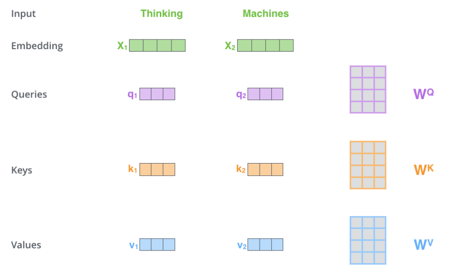
For each input vector (the first layer is the word embeddings, and the other layers are the outputs from the previous layer), we first need to generate three new vectors Q, K, and V, representing the Query vector, Key vector, and Value vector, respectively. Q indicates that to encode the current word, we need to focus on (attend to) other words (including itself). The Key vector can be thought of as the key information used for retrieval for this word, while the Value vector is the actual content.
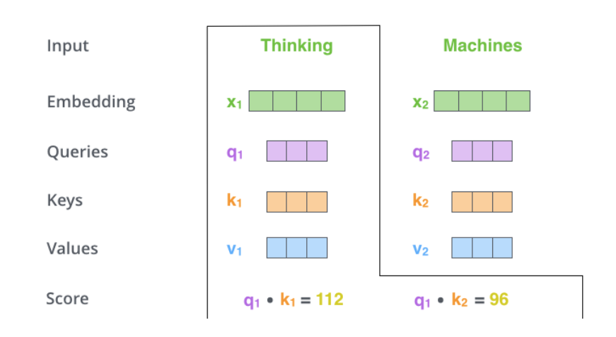
The specific computation process is shown in the figure below. For example, the inputs in the figure are two words ‘thinking’ and ‘machines’. We perform Embedding on them (this is the first layer; if it is a later layer, the input is already the vector), obtaining vectors 𝑥1,𝑥2. Next, we use three matrices to transform them, resulting in vectors 𝑞1,𝑘1,𝑣1 and 𝑞2,𝑘2,𝑣2. For example, 𝑞1=𝑥1𝑊𝑄, where the shape of 𝑥1 is 1×4, and 𝑊𝑄 is 4×3, resulting in 𝑞1 being 1×3. Other computations are similar; to enable the Key and Query to be dot-multiplied, we require that the shapes of 𝑊𝐾 and 𝑊𝑄 be the same, but we do not require 𝑊𝑉 to be the same as them (although the actual implementation in the paper is the same).
After calculating 𝑄𝑡,𝐾𝑡,𝑉𝑡 for each moment t, we can compute Self-Attention. Taking the first moment as an example, we first calculate the dot product of 𝑞1 and 𝑘1,𝑘2 to get the score, as shown in the figure below.
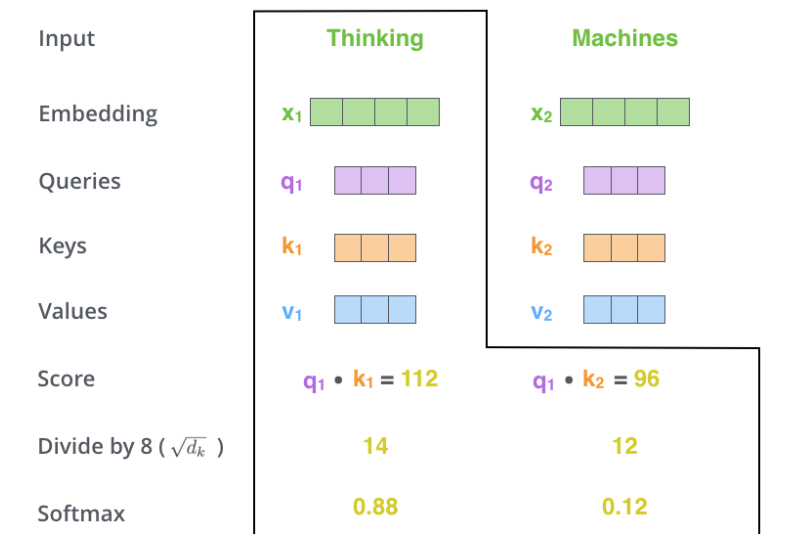
Next, we use softmax to convert the scores into probabilities. Note that the scores are divided by 8 (𝑑𝑘) before calculating the softmax. According to the paper, this makes the gradient calculation more stable. The calculation process is shown in the figure below.
Next, we perform a weighted average of all moments’ V using the probabilities obtained from softmax. This means that the resulting vector comprehensively considers the input information from all moments according to Self-Attention probabilities, as shown in the figure below.
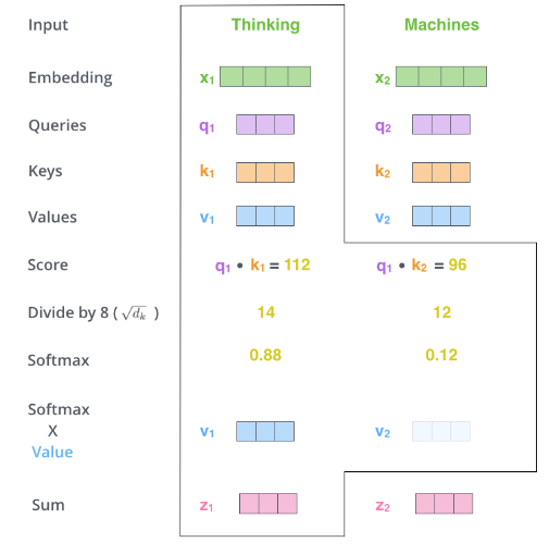
This only demonstrates the computation process for the first moment; the process for other moments is completely the same.
Softmax example code:
import numpy as np

def softmax(x):
    """Compute softmax values for each sets of scores in x."""
    # e_x = np.exp(x)
    e_x = np.exp(x)
    return e_x / e_x.sum()

if __name__ == '__main__':
    x = np.array([-3, 2, -1, 0])
    res = softmax(x)
    print(res)                        # [0.0056533  0.83902451 0.04177257 0.11354962]
It is important to note that the above process can be computed in parallel.
Multi-Head Attention
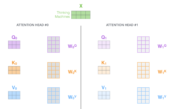
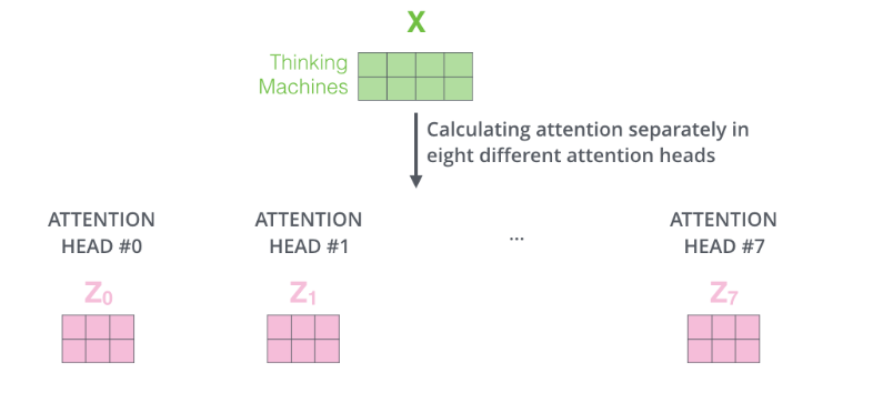
The paper also introduced the concept of Multi-Head Attention. It’s quite simple: the previously defined set of Q, K, and V allows a word to attend to related words. We can define multiple sets of Q, K, and V, which can focus on different contexts. The process of calculating Q, K, and V remains the same, but now the transformation matrices change from a single set (𝑊𝑄,𝑊𝐾,𝑊𝑉) to multiple sets (𝑊𝑄0,𝑊𝐾0,𝑊𝑉0), (𝑊𝑄1,𝑊𝐾1,𝑊𝑉1), as shown in the figure below.
For the input matrix (time_step, num_input), each set of Q, K, and V can produce an output matrix Z (time_step, num_features), as shown in the figure below.
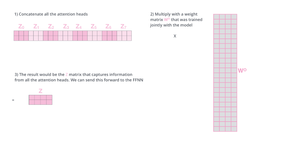
However, the subsequent fully connected network requires the input to be a single matrix rather than multiple matrices. Therefore, we can concatenate the outputs of multiple heads along the second dimension, but this results in some redundancy in features, so the Transformer uses a linear transformation (matrix 𝑊𝑂) to compress it. The process is shown in the figure below.
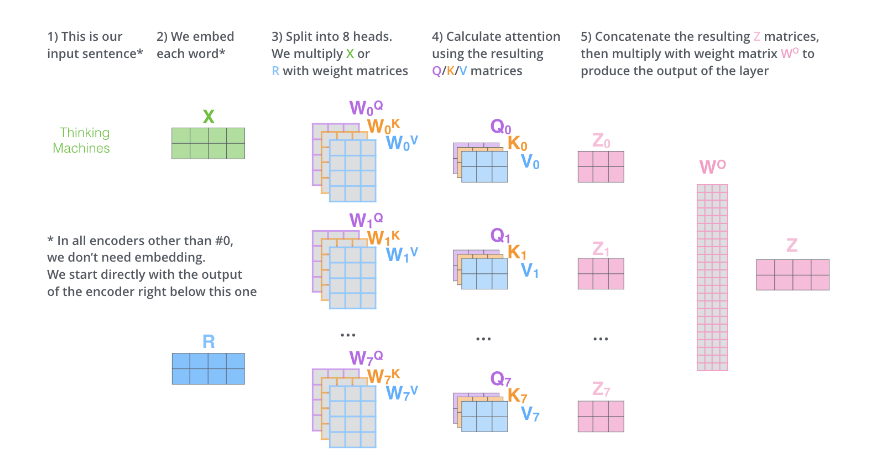
The above steps involve many steps and matrix operations. We will represent the entire process in a single diagram, as shown in the figure below.
We have learned the Self-Attention mechanism of the Transformer. Next, we will look at a specific example to see what kind of semantics different Attention Heads have learned.

The comparison of the above two figures also shows the benefits of using multiple Heads—each Head (driven by the data) learns different semantics.
Positional Encoding
Our goal is to use Self-Attention to replace RNNs. RNNs can remember past information, which can be equivalently (or even better) achieved by Self-Attention’s real-time attention to any relevant word. RNNs also have a specific capability to consider the order (positional) relationships of words. For example, even if the words are exactly the same, the semantics may be completely different, such as ‘the ticket from Beijing to Shanghai’ and ‘the ticket from Shanghai to Beijing’; they have significant semantic differences. The Self-Attention we introduced above does not consider the order of words. If the model parameters are fixed, both instances of ‘Beijing’ in the above sentences would be encoded into the same vector. However, in reality, we would expect the results of encoding these two instances of ‘Beijing’ to be different; the former may need to encode the departure city’s semantics, while the latter needs to include the destination city’s semantics. RNNs can potentially learn this, but the cost of RNNs is sequential processing, making parallelization difficult.
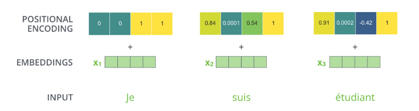
To solve this problem, we need to introduce positional encoding, meaning that the input at time t, in addition to the embedding (which is position-independent), also includes a vector that is position-dependent. We add the embedding and the positional encoding vector together as the model input. Thus, if two words appear at different positions, even though their embeddings are the same, the resulting vectors will be different due to the different positional encodings.
There are many methods for positional encoding, one important factor to consider is that it should encode the relative positional relationships. For example, in the two sentences: ‘the ticket from Beijing to Shanghai’ and ‘Hello, we want a ticket from Beijing to Shanghai.’ Clearly, after adding positional encoding, the vectors for the two instances of ‘Beijing’ will be different, and the vectors for the two instances of ‘Shanghai’ will also be different. However, we expect Query (Beijing1) Key (Shanghai1) to equal Query (Beijing2) Key (Shanghai2). The specific encoding algorithm will be introduced in the code section. The model after adding positional encoding is shown in the figure below.
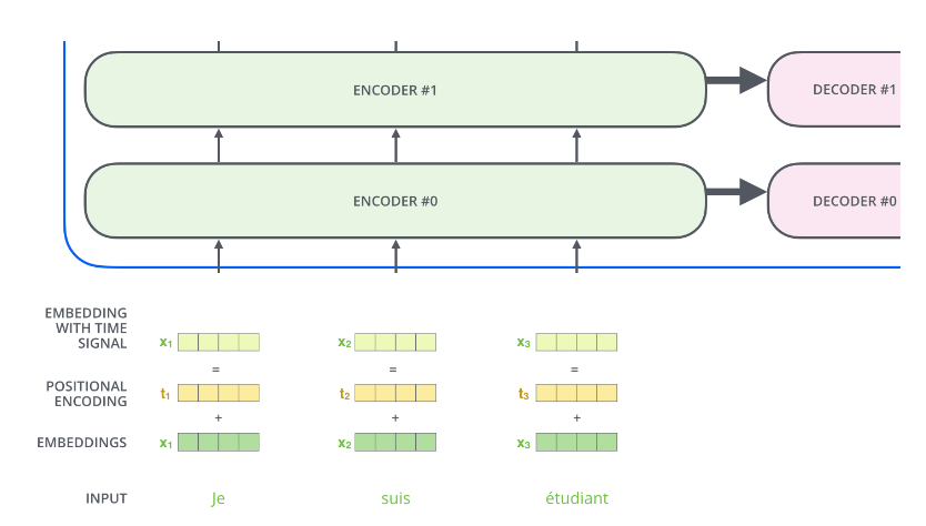
An example of specific positional encoding is shown in the figure below.
Residual Connections and Normalization
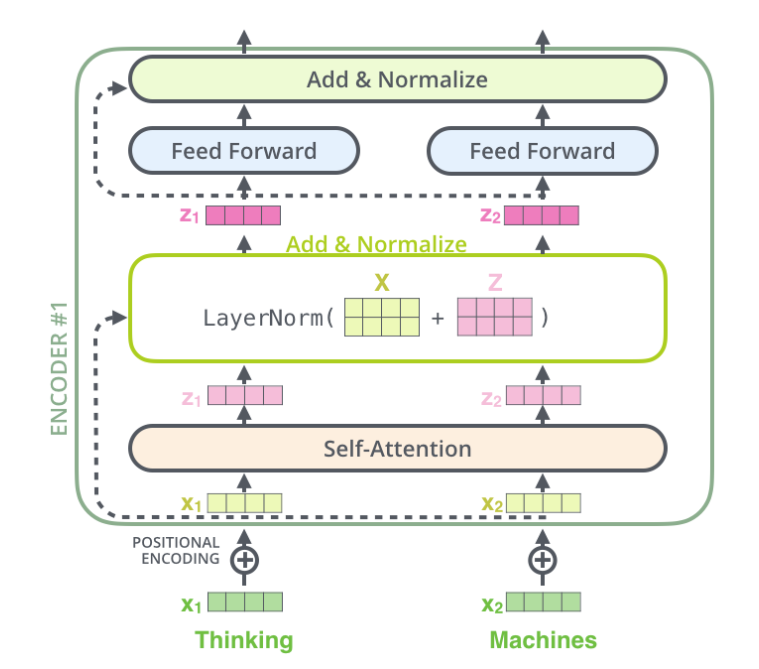
Each Self-Attention layer will add a residual connection followed by a LayerNorm layer, as shown in the figure below.
The figure below shows more details: the inputs 𝑥1,𝑥2 after the self-attention layer become 𝑧1,𝑧2, then they are added to the inputs of the residual connection 𝑥1,𝑥2, and then output to the fully connected layer after passing through the LayerNorm layer. The fully connected layer also has a residual connection and a LayerNorm layer, and finally outputs to the previous layer.
The Decoder is similar to the Encoder, as shown in the figure below, with the difference being that it has an additional Encoder-Decoder Attention layer. The input to this layer comes from the Self-Attention layer and also from the outputs of all moments from the last layer of the Encoder. The Query for the Encoder-Decoder Attention layer comes from the previous layer, while the Key and Value come from the outputs of the Encoder.
Additionally, in the attention layer of the decoder, the use of masks is crucial to ensure that the decoder can only use information from the source language sentence and the previously generated target words when generating each target word.
Pytorch Implementation of Transformer
import torch
import torch.nn as nn
import math

# Positional encoding module
class PositionalEncoding(nn.Module):
    def __init__(self, d_model, max_len=5000):
        super(PositionalEncoding, self).__init__()
        pe = torch.zeros(max_len, d_model)
        position = torch.arange(0, max_len, dtype=torch.float).unsqueeze(1)
        div_term = torch.exp(torch.arange(0, d_model, 2).float() * (-math.log(10000.0) / d_model))
        pe[:, 0::2] = torch.sin(position * div_term)
        pe[:, 1::2] = torch.cos(position * div_term)
        pe = pe.unsqueeze(0)
        self.register_buffer('pe', pe)

    def forward(self, x):
        x = x + self.pe[:x.size(0), :]
        return x

# Transformer model
class TransformerModel(nn.Module):
    def __init__(self, ntoken, d_model, nhead, d_hid, nlayers, dropout=0.5):
        super(TransformerModel, self).__init__()
        self.model_type = 'Transformer'
        self.pos_encoder = PositionalEncoding(d_model)
        self.encoder = nn.Embedding(ntoken, d_model)
        self.transformer = nn.Transformer(d_model, nhead, d_hid, nlayers, dropout)
        self.decoder = nn.Linear(d_model, ntoken)
        self.init_weights()
        self.dropout = nn.Dropout(dropout)

    def generate_square_subsequent_mask(self, sz):
        # Generate subsequent mask to prevent information leakage
        mask = (torch.triu(torch.ones(sz, sz)) == 1).transpose(0, 1)
        mask = mask.float().masked_fill(mask == 0, float('-inf')).masked_fill(mask == 1, float(0.0))
        return mask

    def init_weights(self):
        # Initialize weights
        initrange = 0.1
        self.encoder.weight.data.uniform_(-initrange, initrange)
        self.decoder.bias.data.zero_()
        self.decoder.weight.data.uniform_(-initrange, initrange)

    def forward(self, src, src_mask):
        # Forward propagation
        src = self.encoder(src) * math.sqrt(self.d_model)
        src = self.pos_encoder(src)
        output = self.transformer(src, src, src_key_padding_mask=src_mask)
        output = self.decoder(output)
        return output

# Example usage
ntokens = 1000  # Vocabulary size
d_model = 512  # Embedding dimension
nhead = 8  # Number of heads in multi-head attention
d_hid = 2048  # Dimension of feedforward network model
nlayers = 6  # Number of layers
dropout = 0.2  # Dropout rate

model = TransformerModel(ntokens, d_model, nhead, d_hid, nlayers, dropout)
# Example input
src = torch.randint(0, ntokens, (10, 32))  # (sequence length, batch size)
src_mask = model.generate_square_subsequent_mask(10)  # Create mask
output = model(src, src_mask)
print(output)
Inference Process
In the machine translation task of the Transformer model, the process for the decoder to generate the first translated word (usually referred to as the first target word) is as follows:
1. Start Symbol: At the beginning of the input sequence for the decoder, a special start symbol, such as <sos> (Start Of Sentence), is usually added. This symbol tells the model to begin the translation process.
2. Initialize Hidden State: The hidden state of the decoder is typically initialized to a zero vector or obtained from the output of the last layer of the encoder. This hidden state will be updated at each step of generating the sequence.
3. First Iteration: In the first iteration, the input to the decoder contains only the start symbol <sos>. The decoder generates the first word through the following steps:
• The start symbol is converted into an embedding vector through the embedding layer.
• This embedding vector is input to the first attention layer of the decoder along with the output of the encoder.
• In the self-attention layer, a causal mask (Look-ahead Mask) is used to ensure that the decoder can only attend to the current position and the previous words (in this example, only the start symbol).
• In the encoder-decoder attention layer, the decoder can view the entire output of the encoder since this is the first iteration, and it needs to gather information about the entire source language sentence.
• After passing through the feedforward network of the decoder, the output layer generates a probability distribution representing the next possible word.
• The word with the highest probability is chosen as the first translated word, or decoding strategies such as greedy search or beam search can be used to select the word.
4. Subsequent Iterations: Once the first word is generated, it will be added to the input sequence of the decoder, along with <sos>, as input for the next step. In subsequent iterations, the decoder will continue to generate the next word until it encounters an end symbol <eos> or reaches the maximum sequence length.
During the training phase, the true words of the target sequence (including <sos> and <eos>) will be used to compute the loss function and update the model’s weights through backpropagation. During the inference phase, the decoder gradually generates translations using the above process until a complete sentence is formed.