Source: AI Technology Online
Transformer. I would call it the best article explaining the Transformer model.The article mainly introduces the specific implementation of the Transformer model:
-
Overall Architecture of Transformer -
Overview of Transformer -
Introduction to Tensors -
Self-Attention Mechanism -
Multi-Head Attention Mechanism -
Position-wise Feed-Forward Networks -
Residual Connections and Layer Normalization -
Positional Encoding -
Decoder -
Masks: Padding Mask + Sequence Mask -
Final Linear Layer and Softmax Layer -
Embedding Layer and Final Linear Layer -
Regularization Operations
Blog Address: https://blog.csdn.net/benzhujie1245com/article/details/117173090
English Address: http://jalammar.github.io/illustrated-transformer/
The article is a bit long, so it’s recommended to bookmark it.
1. Transformer Model Architecture
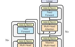
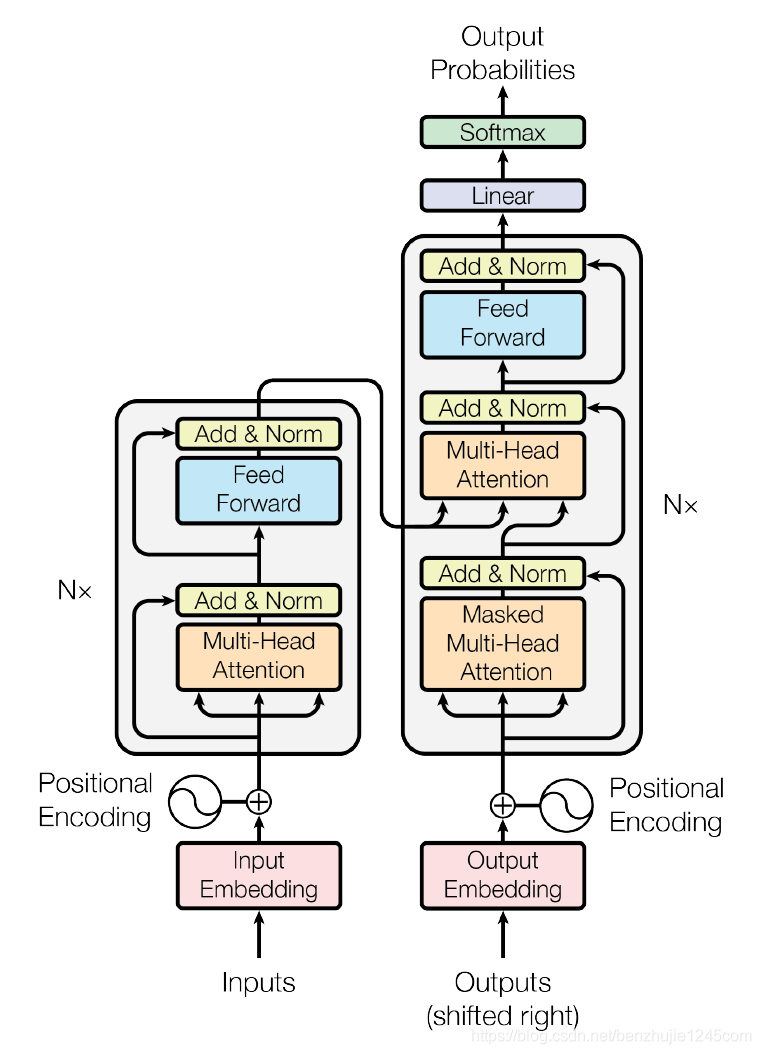
In 2017, Google proposed the Transformer model in the paper Attention is All You Need (Paper Address: https://arxiv.org/abs/1706.03762), which uses the Self-Attention structure to replace the commonly used RNN network structure in NLP tasks.
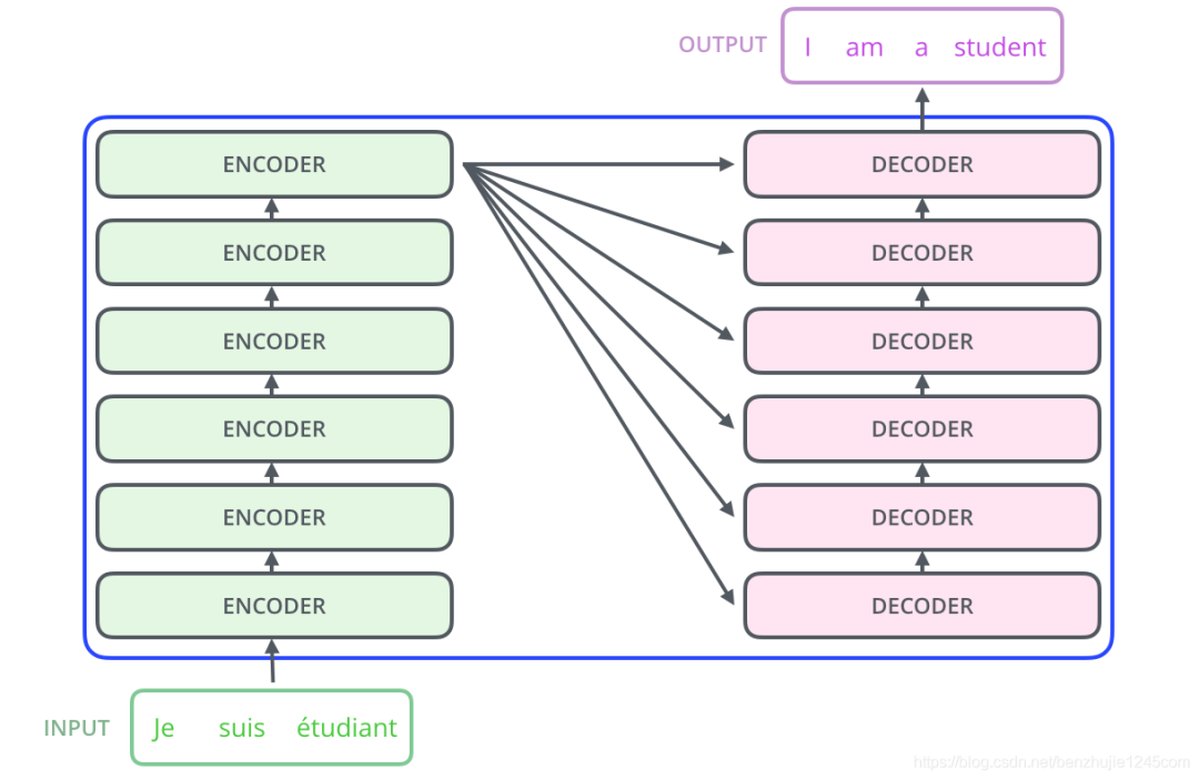
Compared to the RNN structure, its biggest advantage is the ability to perform parallel computations. The overall model architecture of Transformer is shown in the figure:
2. Overview of Transformer
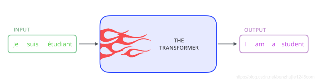
First, let’s view the Transformer model as a black box, as shown in the figure. In machine translation tasks, a sentence in one language is taken as input, and then translated into a sentence in another language as output:
2.1 Encoder-Decoder
The Transformer is essentially an Encoder-Decoder architecture. Therefore, the middle part of the Transformer can be divided into two parts: Encoding Component and Decoding Component
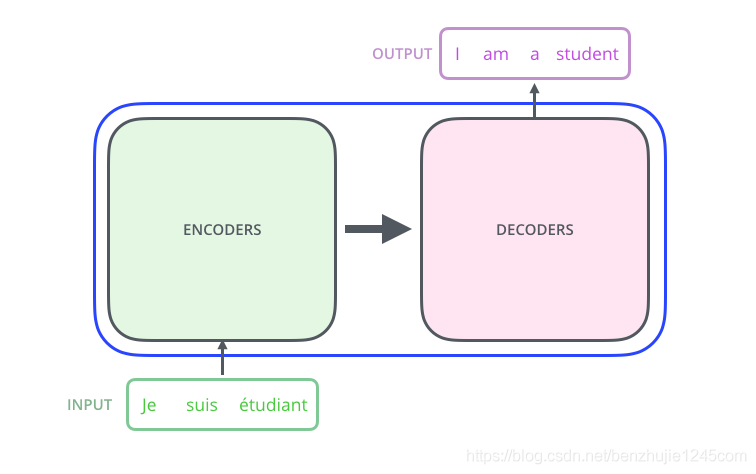
The encoding component consists of multiple layers of encoders (in the paper, the authors used 6 layers of encoders; you can try other numbers of layers in practical use). The decoding component also consists of the same number of decoders (the paper also used 6 layers).
Composition of Encoder/Decoder
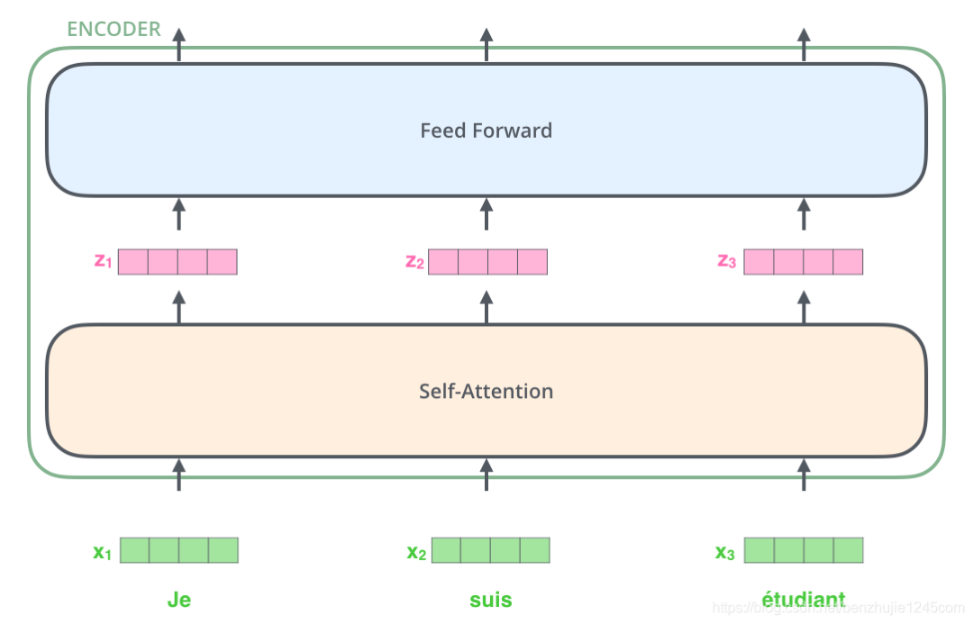
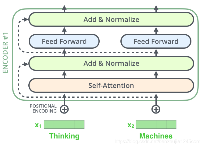
Each encoder consists of two sub-layers:
-
Self-Attentionlayer (self-attention layer) -
Position-wise Feed Forward Network(feedforward network, abbreviated asFFN)
As shown in the figure below: each encoder has the same structure, but they use different weight parameters (the architecture of the 6 encoders is the same, but the parameters are different)
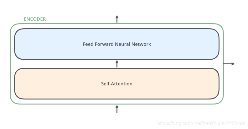
The input to the encoder first flows into the Self-Attention layer. It allows the encoder to use information from other words in the input sentence while encoding a specific word (can be understood as: when we translate a word, we not only focus on the current word but also pay attention to the information of other words).
Note: Focus on the contextual environment of words, not just the words themselves.
Later, we will introduce the internal structure of Self-Attention in detail. Then, the output of the Self-Attention layer flows into the feedforward network.
The decoder also has these two layers from the encoder, but there is also an attention layer (i.e., Encoder-Decoder Attention) that helps the decoder focus on the relevant parts of the input sentence (similar to the attention in the seq2seq model).
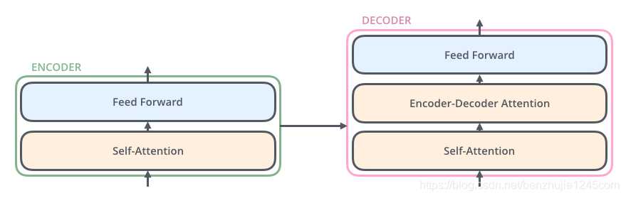
Encoder:
self-attentionlayer + feedforward networkFFN (Position-wise Feed Forward Network)Decoder:
self-attentionlayer +Encoder-Decoder Attention+ feedforward networkFFN (Position-wise Feed Forward Network)
3. Introduction to Tensors
Now that we have understood the main components of the model, let’s start studying various vectors/tensors, and how they flow between these components to convert input through the trained model into output.
3.1 Introduction to Word Embeddings
Like typical NLP tasks, we first use word embedding algorithms (Embedding) to convert each word into a word vector.
In the Transformer paper, the dimension of the word embedding vector is 512.
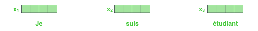
Each word is embedded into a vector of size
512. We will use these simple boxes to represent these vectors.
Word embedding only occurs in the bottom encoder. All encoders will receive a list of vectors of size 512:
-
The bottom encoder receives the word embedding vectors. -
The other encoders receive the output from the previous encoder.
The size of this list is a hyperparameter that we can set—essentially, this parameter is the length of the longest sentence in the training dataset.
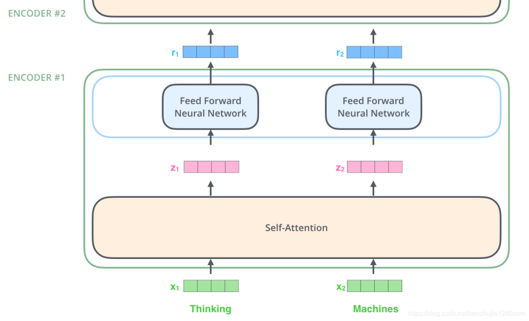
3.2 Encoding After Word Embedding
After completing the embedding operation on the input sequence, each word will flow through the two layers of the encoder.
Next, we will use a shorter sentence as an example to illustrate what happens in each sub-layer of the encoder.
As mentioned above, the encoder receives a vector as input. The encoder first passes these vectors to the Self-Attention layer, then to the feedforward network, and finally passes the output to the next encoder.
4. Self-Attention
4.1 Overview of Self-Attention
First, let’s intuitively understand Self-Attention through an example. Suppose we want to translate the following sentence:
The animal didn’t cross the street because it was too tired
What does it refer to in this sentence? Is it referring to animal or street? For humans, this is a simple question, but for algorithms, it is not so straightforward.
When the model processes it, the Self-Attention mechanism allows it to associate it with animal.
When the model processes each word (each position in the input sequence), the Self-Attention mechanism enables the model to focus not only on the word at the current position but also on words at other positions in the sentence, thus better encoding this word.
If you are familiar with Recurrent Neural Networks RNN, think about how to maintain the hidden state to merge the representations of previously processed words/vectors with the currently processed word/vector. The Transformer uses the Self-Attention mechanism to incorporate the understanding of other words into the current word.
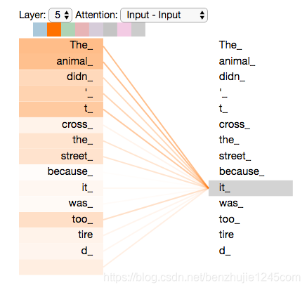
it in Encoder #5 (the top encoder in the stack), some of the attention focuses on The animal and incorporates part of their information into the encoding of it.4.2 Mechanism of Self-Attention
Next, let’s take a look at the specific mechanism of Self-Attention. Its basic structure is shown in the figure:
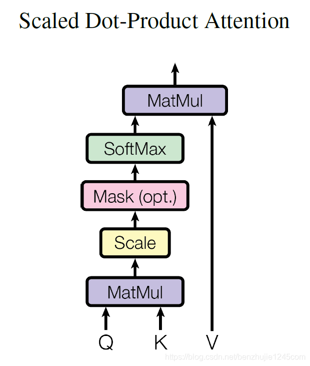
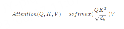
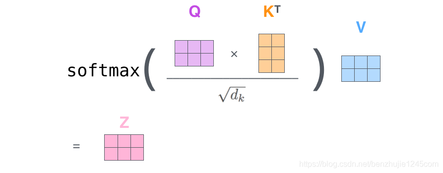
For Self Attention, the Q (Query), K (Key), and V (Value) matrices all come from the same input and are computed as follows:
-
First, compute the dot product between
QandK; to prevent the result from being too large, it is divided by the dimension of theKeyvector. -
Then, use the
Softmaxoperation to normalize the result into a probability distribution, and then multiply by the matrixVto obtain the weighted sum representation.
The entire computation process can be expressed as:
To better understand Self-Attention, let’s go through a specific example in detail.
4.3 Detailed Explanation of Self-Attention
Let’s look at how to calculate Self-Attention using vectors through an example. The steps to calculate Self-Attention are as follows:
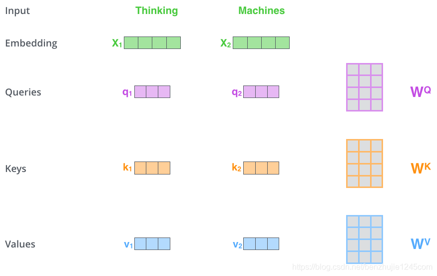
Step 1: Create three vectors for each input vector of the encoder (in this case, each word’s word vector):
-
Queryvector -
Keyvector -
Valuevector
They are obtained by multiplying the word vectors by three matrices that are obtained through training.
Note that the dimensions of these vectors are smaller than the dimensions of the word vectors. The new vectors have a dimension of
64, while the dimensions of theembeddingand encoder input/output vectors are512.The new vectors do not necessarily have to be smaller; this is a structural choice to maintain consistency in multi-head attention calculations.
Query vector associated with that word.Eventually, a Query, a Key, and a Value vector will be created for each word in the input sentence.
What are the
Query, Key, and Valuevectors? They are an abstraction that is very useful for attention calculations and reasoning. Continue reading the attention calculation process below to understand the roles these vectors play.
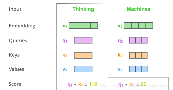
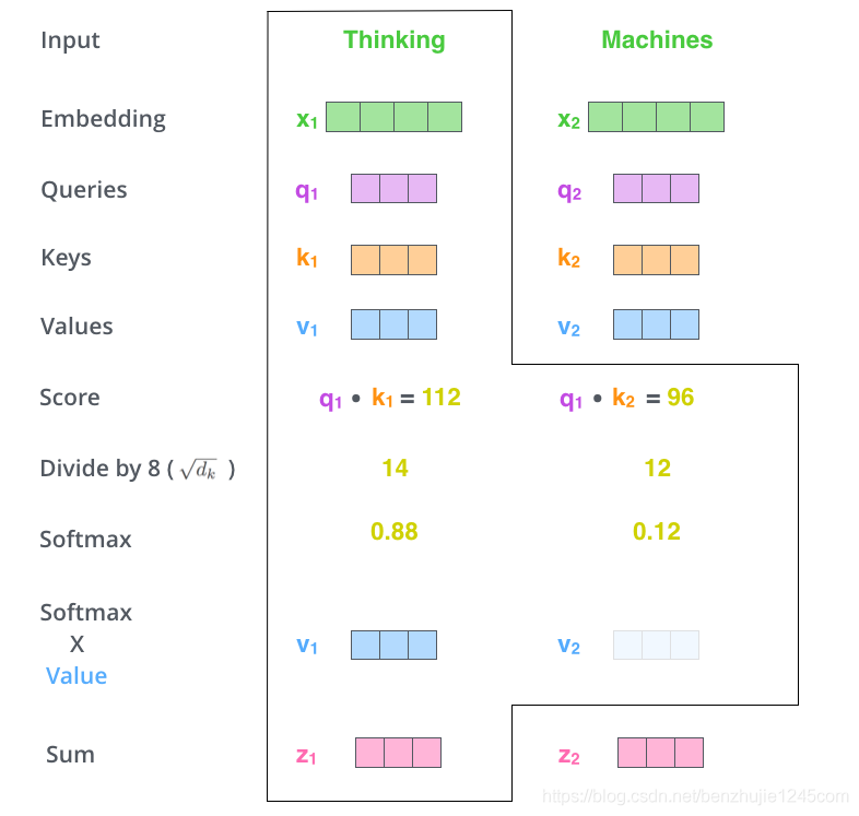
Step 2: Calculate the attention scores.
Assuming we are calculating the self-attention for the first word Thinking in this example, we need to calculate a score for each word in the sentence based on Thinking. These scores determine how much attention we should pay to each word at other positions when encoding Thinking.
These scores are obtained by calculating the dot product of the Query vector of Thinking with the Key vectors of the words that need to be scored. If we calculate the attention score for the first position word in the sentence, the first score is the dot product with itself, and the second score is the dot product with the next word.
Step 3: Divide each score by the dimension of the Key vector.
The purpose is to make the gradients more stable during backpropagation. In practice, you can also divide by other numbers.
Step 4: Apply the Softmax operation to these scores. Softmax normalizes the scores so that they are all positive and sum to 1.
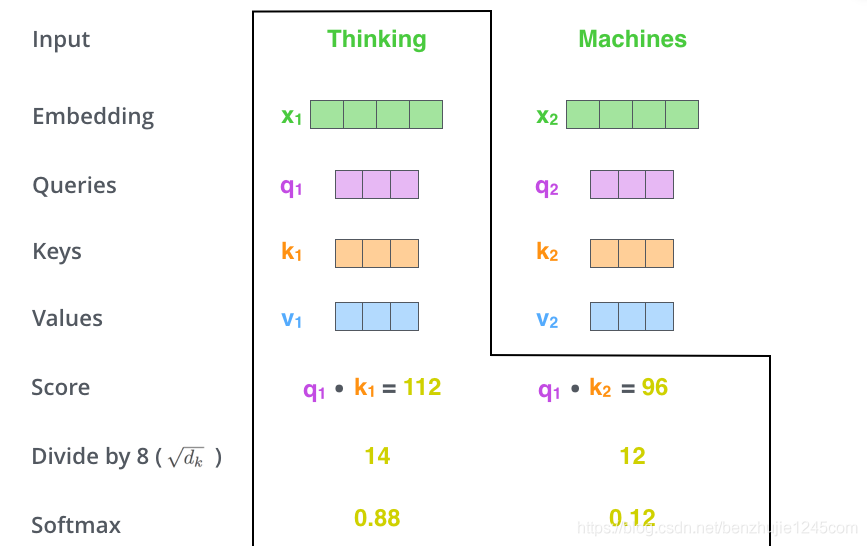
These Softmax scores determine how much attention to place on each word when encoding the word at the current position. Clearly, the word at the current position has the highest score, but sometimes it is useful to pay attention to words related to the current position.
Step 5: Multiply each Softmax score by its corresponding Value vector.
The intuition behind this is: for positions with high scores, the multiplied values will be larger, so we pay more attention to them; for positions with low scores, the multiplied values will be smaller, and we can ignore those words.
The larger, the more emphasis.
Step 6: Sum the weighted Value vectors (the vectors obtained from the previous step). This gives us the output of the self-attention layer at this position.
This completes the calculation of self-attention. The resulting vector will be input into the feedforward network. However, in practical implementations, this calculation is performed in matrix form for faster processing. Next, let’s see how to use matrix calculations.
4.4 Using Matrix to Calculate Self-Attention
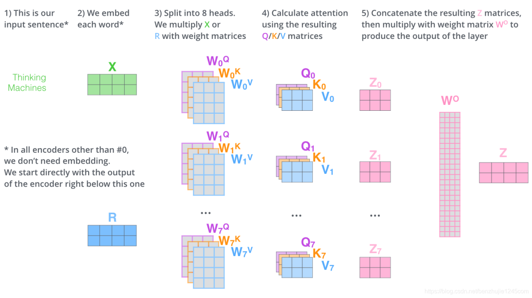
Step 1: Calculate the Query, Key, and Value matrices.
First, place all word vectors into a matrix X, and then multiply by the three weight matrices we trained to obtain the Q, K, V matrices.
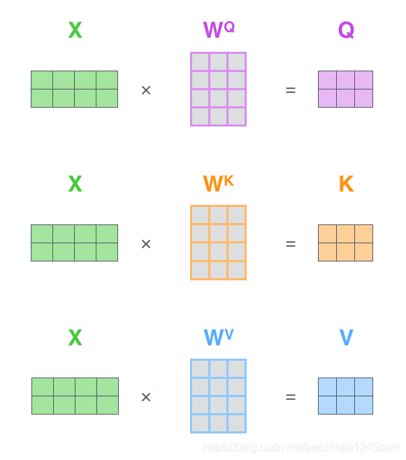
-
Each row in matrix X represents the word vector of each word in the input sentence (length 512, represented by 4 boxes in the figure). -
Each row in matrices Q, K, and V represents the Queryvector,Keyvector, andValuevector respectively (all with a length of 64, represented by 3 boxes in the figure).
Step 2: Calculate self-attention. Since we are using matrices for calculations, we can compress Steps 2 to 6 from above into one step.
5. Multi-Head Attention Mechanism
5.1 Architecture of Multi-Head Attention
In the Transformer paper, a multi-head attention mechanism was added to further enhance the self-attention layer. The specific approach is:
-
First, apply different linear transformations to the Query, Key, andValue; -
Then, concatenate the different Attentionresults; -
Finally, perform another linear transformation.
The basic structure is shown in the figure:
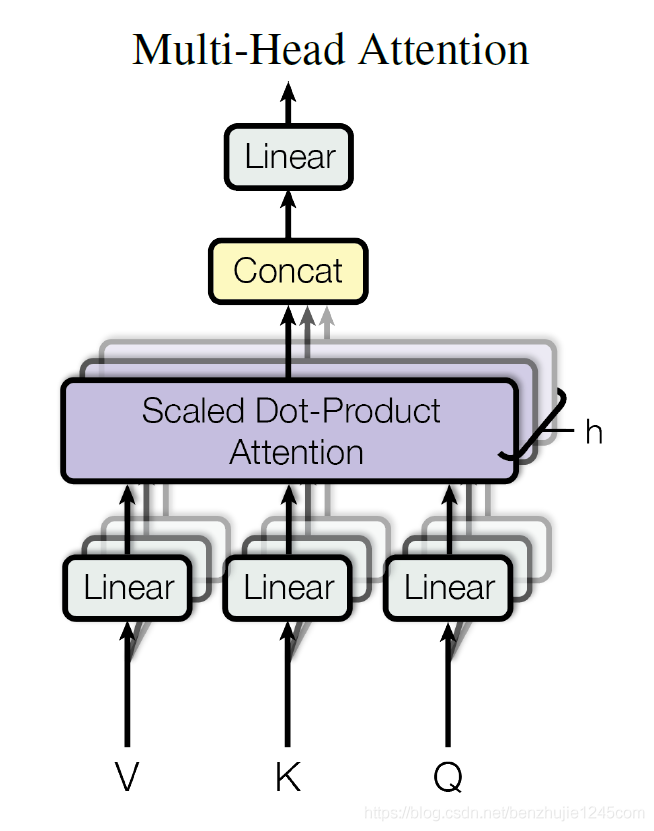
Each group of attention is used to map the input to different sub-representation spaces, allowing the model to focus on different positions in different sub-representation spaces. The entire calculation process can be expressed as:
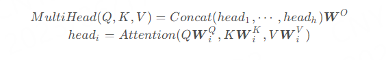
In the paper, it specifies h=8, meaning 8 attention heads are used.
Under multi-head attention, we maintain different Query, Key, and Value weight matrices for each group of attention, resulting in different Query, Key, and Value matrices.
As mentioned earlier, we will multiply the input by the Q, K, V matrices to obtain the Query, Key, Value matrices.
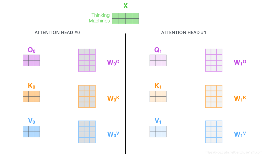
By using different weight matrices, we can perform self-attention calculations 8 times to obtain 8 different Attention matrices.
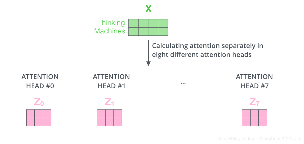
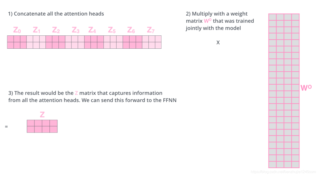
Next, it gets a bit complicated. The feedforward neural network layer receives one matrix (the word vector for each word), not the 8 matrices above. Therefore, we need a way to consolidate these 8 matrices into one matrix. The specific method is as follows:
-
Concatenate the 8 matrices; -
Multiply the concatenated matrix by another weight matrix; -
Obtain the final matrix, which contains all the information from the attention heads, and this matrix will be input into the FFN layer.
5.2 Summary of Multi-Head Attention
This is essentially all about multi-head attention. Below, we will put everything into one diagram for a unified view:
Now let’s revisit the earlier example and see where different attention heads focus when encoding the word it in the example sentence:
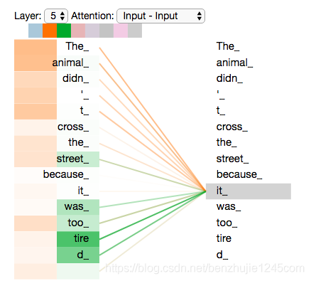
itWhen we encode it, one attention head focuses on The animal, while another focuses on tired. In a sense, the representation of it by the model incorporates parts of the representations of animal and tired.
The essence of Multi-head Attention is: while keeping the total number of parameters unchanged, the same Query, Key, Value are mapped into different subspaces of the original high-dimensional space for attention calculations, and finally, the information captured in different subspaces is merged in the last step.
This reduces the dimensionality of each vector when calculating the Attention for each head, which in some sense prevents overfitting.
Since Attention has different distributions in different subspaces, Multi-head Attention essentially seeks the relationships between sequences from different angles and integrates the relationships captured in different subspaces during the final concatenation step.
6. Position-wise Feed-Forward Networks
Position-wise feed-forward networks are a fully connected feed-forward network, where each word at each position passes through the same feed-forward neural network.
It consists of two linear transformations, i.e., two fully connected layers, with the activation function of the first fully connected layer being the ReLU activation function. It can be expressed as:
In each encoder and decoder, although the structure of this fully connected feed-forward network is the same, the parameters are not shared. The input and output dimensions of the entire feed-forward network are the same, while the output of the first fully connected layer and the input dimension of the second fully connected layer are
7. Residual Connections and Layer Normalization
There is a detail to note in the encoder structure: each sub-layer of each encoder (the Self-Attention layer and the FFN layer) has a residual connection, followed by a layer normalization operation. The entire computation process can be expressed as:
The above operation also applies to the sub-layers of the decoder. Assuming a Transformer consists of 2 layers of encoders and 2 layers of decoders, it is shown in the figure below:
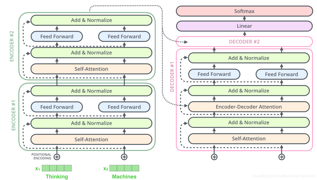
To facilitate residual connections, the output dimensions of all sub-layers and embedding layers in the encoder and decoder need to remain consistent, as specified in the Transformer paper.
8. Positional Encoding
So far, we have described a model that lacks one thing: a method to represent the order of words in the sequence. To solve this problem, the Transformer model adds a vector to each input word embedding vector.
These vectors follow a specific pattern learned by the model, helping the model determine the position of each word or the distance between different words in the sequence.
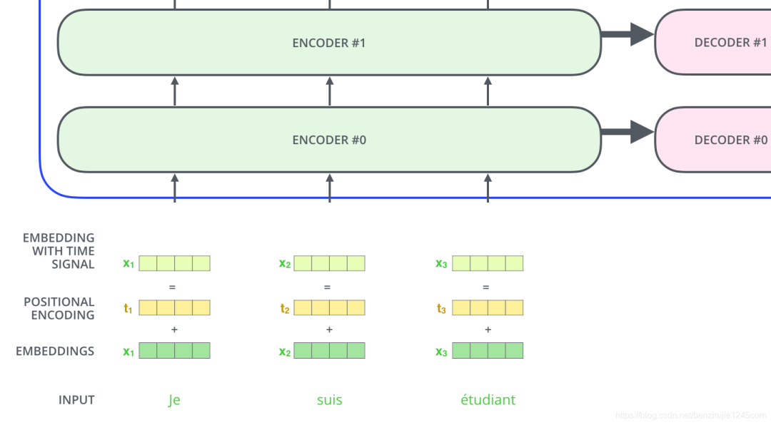
If we assume the dimension of the word embedding vector is 4, the actual positional encoding is as follows:
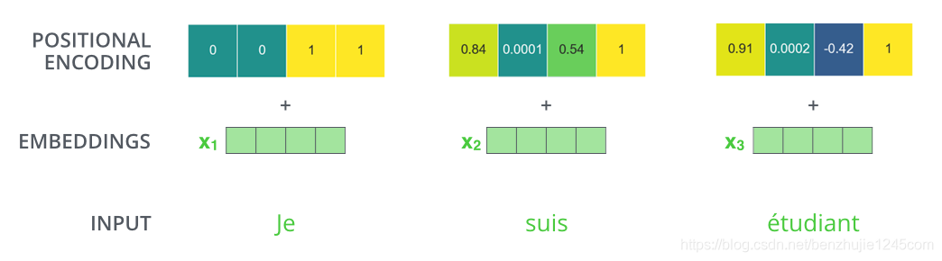
What pattern do positional encoding vectors follow? The specific mathematical formula is as follows:
Where represents the position and represents the dimension. The above function allows the model to learn the relative positional relationships between: Any position can be represented as a linear function of:
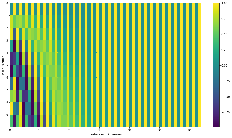
In the figure below, we visualize these values. Each row corresponds to the positional encoding of a vector at a position. So the first row corresponds to the positional encoding of the first word in the input sequence. Each row contains 64 values, each ranging between -1 and 1.
It is important to note that the official provided example code (the get_timing_signal_1d() function in the TensorFlow 1.x version and the call() function in the TensorFlow 2.x version) has slight differences from the method in the Transformer paper:
-
In the Transformerpaper, the values generated by thesinefunction andcosinefunction are interleaved; -
In the official provided code, the left half of the values are all generated by the sinefunction, while the right half are all generated by thecosinefunction, and then they are concatenated.
The visualization of the positional encoding values generated by the official code is as follows:
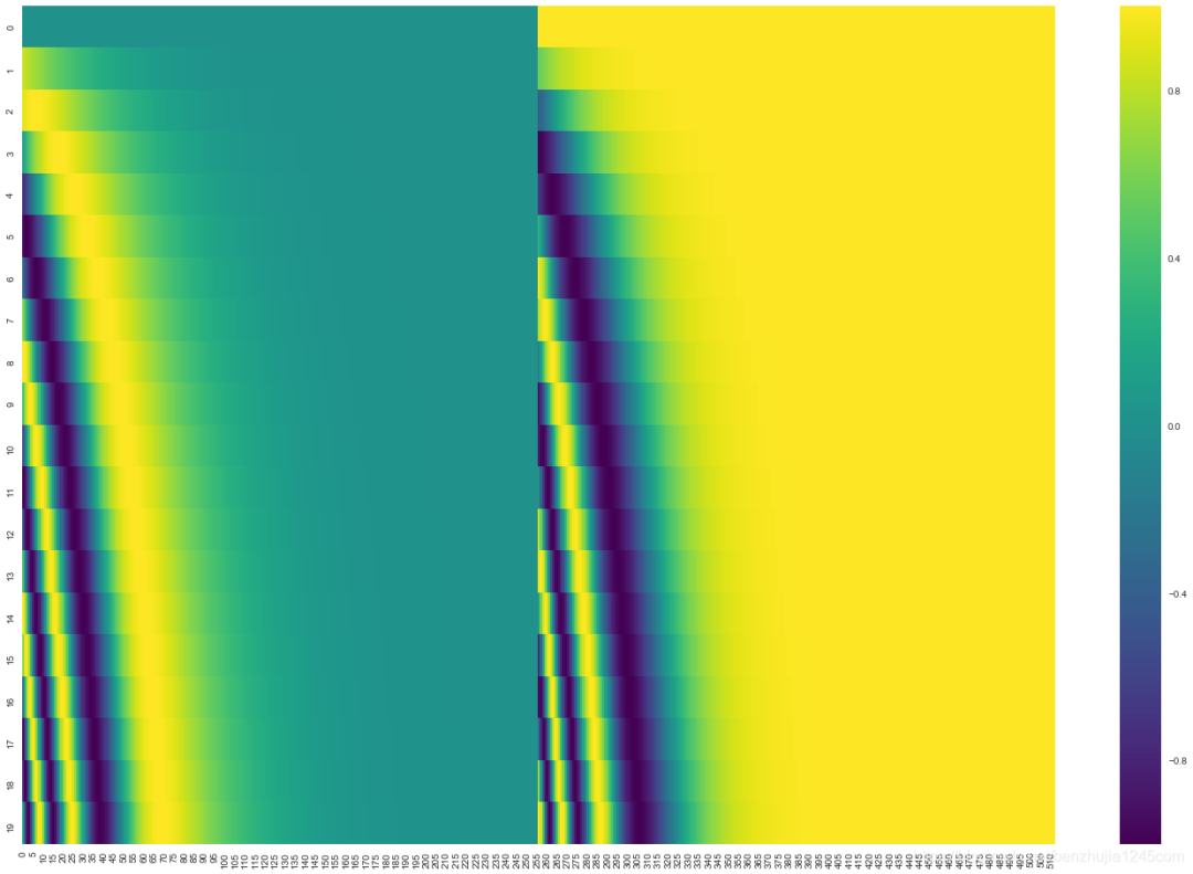
This is not the only way to generate positional encoding. However, the advantage of this method is that it can be extended to unknown sequence lengths. For example, when a trained model is asked to translate a sentence that is longer than any sentence in the training set.
9. Decoder
Now that we have introduced most of the concepts of the encoder, we also understand how the components of the decoder work. Now let’s look at how the encoder and decoder work together.
From the previous introduction, we know that the input to the first encoder is a sequence, and the output of the last encoder is a set of attention vectors Key and Value. These vectors will be used in the Encoder-Decoder Attention layer of each decoder, helping the decoder focus on the appropriate parts of the input sequence.
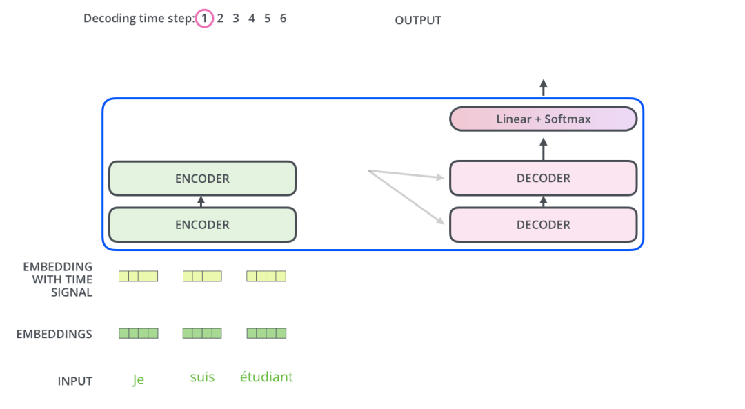
After completing the encoding phase, we begin the decoding phase. Each time step of the decoding phase outputs one element.
This process will be repeated until an end symbol is output, indicating that the Transformer decoder has completed its output. The output of each step will be input into the first decoder of the next time step, and the decoder will display the decoding results just like we processed the encoder input. Just as we add positional encoding to the encoder input, we also add positional encoding to the decoder input to indicate the position of each word.
The Encoder-Decoder Attention layer works similarly to the multi-head self-attention mechanism. The difference is that the Encoder-Decoder Attention layer constructs the Query matrix from the output of the previous layer, while the Key and Value matrices come from the output of the encoder stack.
10. Masks
Mask refers to a mask that covers certain values, preventing them from having an effect during parameter updates. The Transformer model involves two types of mask: Padding Mask and Sequence Mask.
-
Padding Maskis used in allscaled dot-product attention. -
While
Sequence Maskis only used in theSelf-Attentionof the decoderDecoder.
10.1 Padding Mask
What is Padding mask? Since each batch of input sequences has different lengths, we need to align the input sequences.
Specifically: it means padding 0 after shorter sequences (but if the input sequence is too long, it is truncated, discarding the excess directly). Since these padding positions are actually meaningless, our Attention mechanism should not pay attention to these positions, so we need to process them.
The specific approach is to add a very large negative number (negative infinity) to the values at these positions, so that after Softmax, the probabilities at these positions will approach 0.
10.2 Sequence Mask
Sequence Mask is used to ensure that the Decoder cannot see future information. That is, for a sequence, at time step t, our decoding output should only depend on the outputs before time step t, not on the outputs after it. We need a way to hide the information that comes after.
Specifically: generate an upper triangular matrix, where all values above the diagonal are 0. Applying this matrix to each sequence achieves our goal.
In summary: For the Self-Attention of the Decoder, both scaled dot-product attention need Padding Mask and Sequence Mask, and the specific implementation is that the two Mask are added together. In other cases, only Padding Mask is needed.
11. Final Linear Layer and Softmax Layer
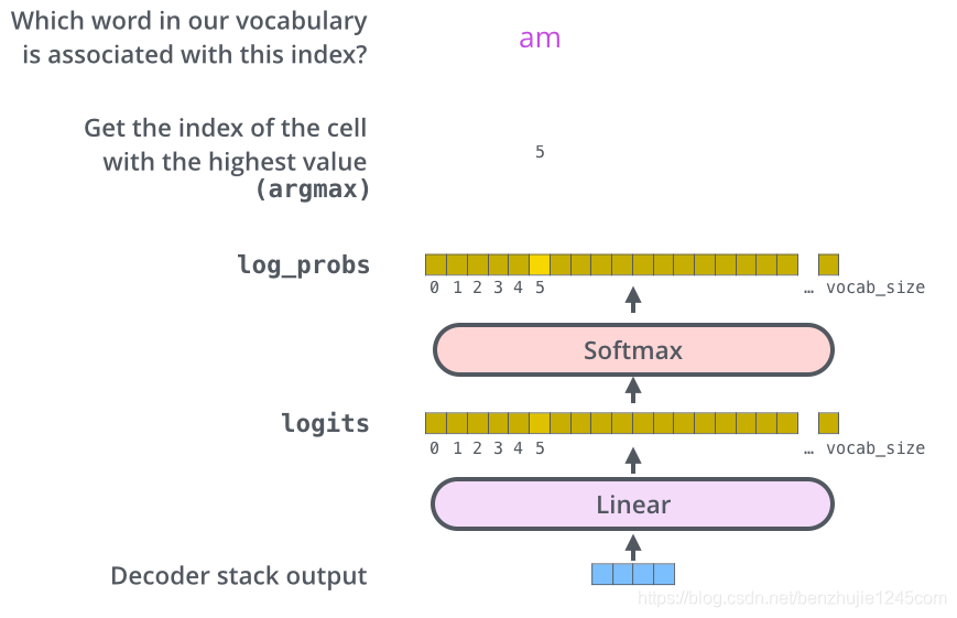
The output of the decoder stack is a float vector. How do we convert this vector into a word? This is achieved through a linear layer followed by a Softmax layer.
11.1 Linear Layer
The linear layer is a simple fully connected neural network that maps the output vector of the decoder stack to a longer vector, known as the logits vector.
11.2 Softmax Layer
Now assume our model has 10000 English words (the output vocabulary of the model). Therefore, the logits vector has 10000 numbers, each representing a score for a word.
Then, the Softmax layer converts these scores into probabilities (converting all scores to positive values that sum to 1). Finally, the word corresponding to the highest probability is selected as the output for this time step.
12. Embedding Layer and Final Linear Layer
In the Transformer paper, there is a detail mentioned: the embedding layers in the encoding and decoding components, as well as the final linear layer share the weight matrices.
It is important to note that in the embedding layer, this shared weight matrix is multiplied by
13. Regularization Operations
To improve the performance of the Transformer model, the following regularization operations are used during training:
-
Dropout. TheDropoutoperation is applied to the output of each sub-layer of the encoder and decoder before performing the residual connection and layer normalization. After the addition of the word embedding vector and positional encoding vector, theDropoutoperation is performed. The parameters provided in theTransformerpaper are -
Label Smoothing. The parameter provided in theTransformerpaper is.
14. References
-
Original English Address: The Illustrated Transformer -
Attention Is All You Need -
Illustrated Transformer -
Detailed Explanation of Transformer (Attention Is All You Need) -
Understanding Language’s Transformer Source: Machine Learning Grocery Store
[Disclaimer] The reproduction is for non-commercial educational and research purposes only, aimed at academic news information dissemination. The copyright belongs to the original author. If there is any infringement, please contact us immediately, and we will delete it promptly.