Common Techniques for Accelerating Transformers

Source: DeepHub IMBA


This article is about 1800 words long, and it is recommended to read in 5 minutes.
This article summarizes some commonly used acceleration strategies.

Transformers is a powerful architecture, but the model can easily encounter OOM (Out of Memory) issues or hit runtime limits of the GPU during training due to its self-attention mechanism, which effectively processes sequential data and captures long-distance dependencies.

This is mainly because:

1. Large number of parameters: Transformer models typically contain a large number of parameters, especially when scaling at the model level (e.g., increasing the number of layers or heads). These parameters require a significant amount of memory to store weights and gradients.

2. Self-attention computation: The self-attention mechanism requires calculating the relationships between each element of the input sequence and all other elements, leading to a significant increase in computational complexity and memory requirements as the input length grows. This is particularly pronounced for very long sequences.

3. Activation and intermediate state storage: During training, intermediate activation states from the forward pass need to be stored for use during backpropagation. This adds additional memory overhead.

To address these issues, we will summarize some commonly used acceleration strategies today.

Fixed-Length Padding

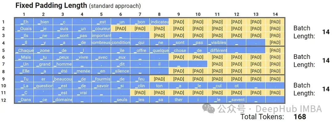
When processing text data, since the lengths of text sequences may vary, many machine learning models (especially Transformer-based models) require input data to have a fixed size. Therefore, it is necessary to apply fixed-length padding to the text sequences.

When using Transformer models, the padding should not affect the model’s learning. Hence, an attention mask is typically used to indicate to the model to ignore these padding positions during self-attention calculations. By implementing this fixed-length padding and corresponding processing methods, Transformer-based models can effectively handle sequences of varying lengths. In practical applications, this method is a common strategy for processing text inputs.

 def fixed_pad_sequences(sequences, max_length, padding_value=0):    padded_sequences = []    for sequence in sequences:        if len(sequence) >= max_length:            padded_sequence = sequence[:max_length] # Trim the sequence if it exceeds max_length        else:            padding = [padding_value] * (max_length - len(sequence)) # Calculate padding            padded_sequence = sequence + padding # Pad the sequence        padded_sequences.append(padded_sequence)    return padded_sequences

This method pads all sequences to a uniform length. While this equalizes the lengths, it may result in many padding instances within a batch due to the original differences in sequence sizes, leading to the dynamic padding strategy.

Dynamic padding dynamically adjusts the input sequences in each batch to the maximum length. Unlike fixed-length padding, where all sequences are padded to match the longest sequence in the entire dataset, dynamic padding fills each sequence in a batch based on the length of the longest sequence in that batch.

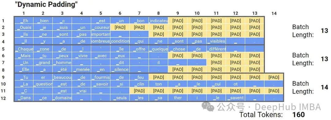
Although each batch has different lengths, the lengths within each batch are uniform, which can speed up processing.

 def pad_sequences_dynamic(sequences, padding_value=0):    max_length = max(len(seq) for seq in sequences) # Find the maximum length in the sequences    padded_sequences = []    for sequence in sequences:        padding = [padding_value] * (max_length - len(sequence)) # Calculate padding        padded_sequence = sequence + padding # Pad the sequence        padded_sequences.append(padded_sequence)    return padded_sequences

Length Matching

Length matching is the process of grouping sequences of similar lengths into batches during training or inference. Length matching is implemented by dividing the dataset into buckets based on sequence length and then sampling batches from these buckets.

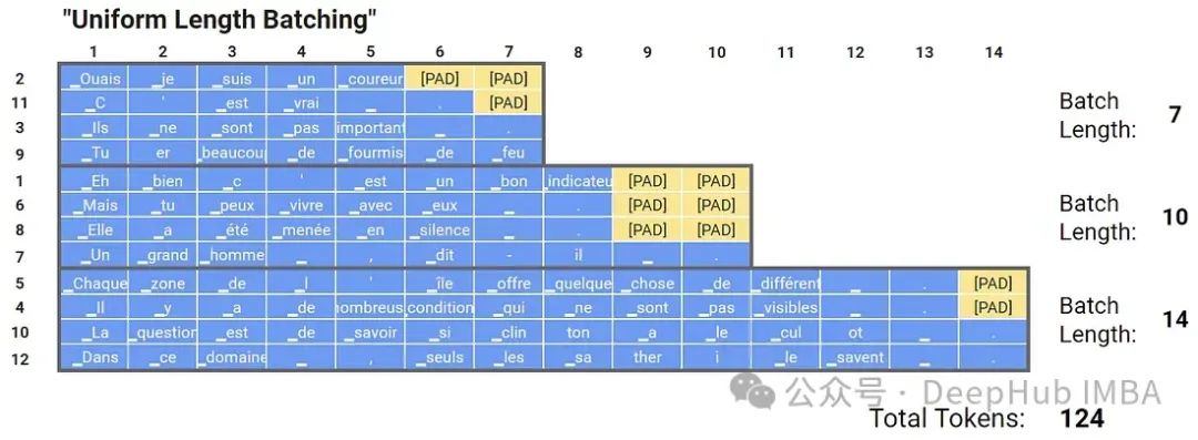
As seen in the above image, the length matching strategy reduces the amount of padding, thus speeding up computation:

 def uniform_length_batching(sequences, batch_size, padding_value=0):    # Sort sequences based on their lengths    sequences.sort(key=len)
    # Divide sequences into buckets based on length    buckets = [sequences[i:i+batch_size] for i in range(0, len(sequences), batch_size)]
    # Pad sequences within each bucket to the length of the longest sequence in the bucket    padded_batches = []    for bucket in buckets:        max_length = len(bucket[-1]) # Get the length of the longest sequence in the bucket        padded_bucket = []        for sequence in bucket:            padding = [padding_value] * (max_length - len(sequence)) # Calculate padding            padded_sequence = sequence + padding # Pad the sequence            padded_bucket.append(padded_sequence)        padded_batches.append(padded_bucket)
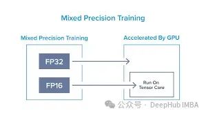
    return padded_batches

Automatic Mixed Precision

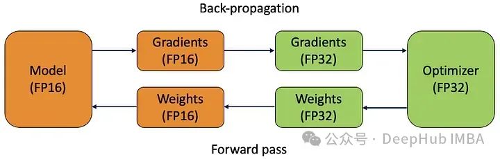
Automatic Mixed Precision (AMP) is a technique for accelerating deep learning model training by using a combination of single precision (float32) and half precision (float16) algorithms. It leverages the capabilities of modern GPUs, allowing for faster computations and reduced memory usage compared to float32.

 import torch from torch.cuda.amp import autocast, GradScaler
 # Define your model model = YourModel()
 # Define optimizer and loss function optimizer = torch.optim.Adam(model.parameters(), lr=1e-3) criterion = torch.nn.CrossEntropyLoss()
 # Create a GradScaler object for gradient scaling scaler = GradScaler()
 # Inside the training loop for inputs, targets in dataloader:    # Clear previous gradients    optimizer.zero_grad()
    # Cast inputs and targets to the appropriate device    inputs, targets = inputs.to(device), targets.to(device)
    # Enable autocasting for forward pass    with autocast():        # Forward pass        outputs = model(inputs)        loss = criterion(outputs, targets)
    # Backward pass    # Scale the loss value    scaler.scale(loss).backward()
    # Update model parameters    scaler.step(optimizer)
    # Update the scale for next iteration    scaler.update()

AMP dynamically adjusts the computational precision during training, allowing the model to use float16 for most computations while automatically promoting certain calculations to float32 to prevent numerical instability issues like underflow or overflow.

Fp16 vs Fp32

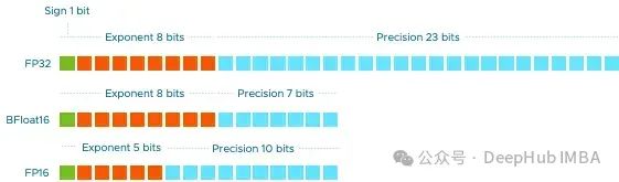
Double precision (FP64) consumes 64 bits. The sign bit is 1, the exponent is 11 bits, and the effective precision is 52 bits.

Single precision (FP32) consumes 32 bits. The sign bit is 1, the exponent is 8 bits, and the effective precision is 23 bits.

Half precision (FP16) consumes 16 bits. The sign bit is 1, the exponent is 5 bits, and the effective precision is 10 bits.

Therefore, FP16 can improve memory savings and significantly speed up model training. Considering the advantages of FP16 and its dominant area of use in model inference tasks, it is well-suited for inference tasks. However, FP16 can lead to numerical precision loss, resulting in inaccurate computed or stored values, which is critical when the precision of these values is essential.

Additionally, this optimizer is tailored for classification tasks; FP16 performs poorly for regression tasks that require precise numerical values.

Conclusion

The methods mentioned above can alleviate memory shortages and computational resource limitations to some extent, but for large models, we still need a powerful GPU.