Building Neural Networks with Numpy Instead of TensorFlow

Produced by Big Data Digest

Author: Jiang Baoshang

Many students, after starting with machine learning, directly use TensorFlow to implement neural networks, with little understanding of the underlying mechanisms of neural networks.

Programming languages and frameworks evolve rapidly, so understanding the principles behind them is essential. Below, we will implement a neural network step by step using Numpy.

This article aims to help everyone organize their knowledge of neural networks, and this is the first part, where we will simply set up a basic framework. We will not cover gradient descent, learning rate tuning, and other topics at this time.

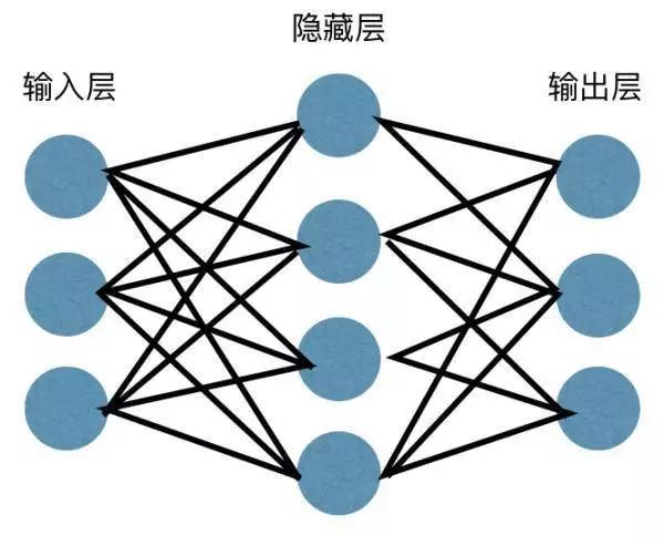
The simplest neural network consists of three elements: the input layer, the hidden layer, and the output layer. Its working mechanism can be completely likened to a meta-function: Y=W*X+b.

A simple neural network can be understood as the input and output of two univariate functions.

First: Y₁=A₁(W₁*X+b₁), where X is the input of the original data, and A₁ represents the activation function.

Second: Y₂=A₂(W₂*Y₁+b₂), where Y₁ is the output of the first stage, and A₂ is the activation function. The parameters W₁, W₂, b₁, and b₂ are generally different.

In this article, we will use two activation functions: one is tanh(x), and the other is softmax. The function curves for both are as follows.

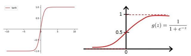
Both functions have the same characteristic: the function values change significantly around zero, while their outputs stabilize as the input moves away from zero.

First, import the relevant libraries, requiring two libraries: one for scientific computing, Numpy, and the other is math.

import numpy as np
import math

Next, define the activation functions,

def tanh(x):    return np.tanh(x)
def softmax(x):   exp=np.exp(x-x.max())   return exp/exp.sum()

These two activation functions include the tanh function, which is directly embedded in Numpy. The softmax function is set according to its mathematical definition. The second activation function, being an exponential function, can vary significantly, so we use x-x.max to reduce its range of variation, which does not affect the result.

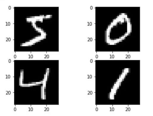
We will use images of size 28*28 pixels. In the future, we will train the network using a handwritten digit dataset, so there will be 10 digit inputs, which are [1,2,3,4,5,6,7,8,9,10]. Therefore, we need to define three lists first.

dinensions=[28*28,10]
activation=[tanh,softmax]
distribution=[{'b':[0,0]},             {'b':[0,0],'w':[-math.sqrt(6/(dinensions[0]+dinensions[1])),math.sqrt(6/(dinensions[0]+dinensions[1]))]}]

The dinensions list contains two numbers: the first is the pixel size of the image, and the second is the change in input for the digits.

The activation list contains two activation functions: tanh and softmax.

The distribution list contains data in dictionary format, corresponding to the range of values for the neural network parameters.

The first layer does not include parameter W.

def init_parameters_b(layer):   dist=distribution[layer]['b']   return np.random.rand(dinensions[layer])*(dist[1]-dist[0])+dist[0]  # Ensures that the generated random numbers are within the range of b
def init_parameters_w(layer):   dist=distribution[layer]['w']   return np.random.rand(dinensions[layer-1],dinensions[layer])*(dist[1]-dist[0])+dist[0]  # Ensures that the generated random numbers are within the range of b

The above code initializes the parameters b and w. Since we are inputting 28*28 numbers and outputting 10 numbers, the first layer’s b also consists of 28*28 numbers. According to matrix multiplication rules, for the second layer, w must have 28*28 rows and 10 columns to satisfy the output of 10 numbers. Therefore, the second layer’s b consists of 10 numbers.

dinensions[X] means slicing, where dinensions[1] returns 10 and dinensions[0] returns 28*28.

Also, because np.random.rand() outputs values in the range [0,1], the parameters in parentheses (i.e., dinensions[layer] just ensure that the output number of values meets the requirement), we set to multiply by (dist[1]-dist[0]) and then add dist[0] to ensure the output values are within the initially set range of b. dist[1] and dist[0] correspond to the upper and lower limits of the parameters.

def init_parameters():   parameters=[]   for i in range(len(distribution)):       layer_parameters={}       for j in distribution[i].keys():           if j=='b':               layer_parameters['b']=init_parameters_b(i)               continue           if j=='w':               layer_parameters['w']=init_parameters_w(i)               continue       parameters.append(layer_parameters)   return parameters

The above code integrates the initialization of the three parameters into one function.

First, we define an empty list (do not mistakenly write it as an empty dictionary) to unify the output of the three parameters.

Note: Dictionary types cannot use append, but lists can, and list.append(dictionary) is also valid.

Then we iterate through distribution starting from zero.Using if statements ensures that all parameters are included.

The second for loop and if statements are for checking and correctly adding parameters.

parameters=init_parameters()   # Assign the parameters to a new variable.
def predict(img,parameters):    I0_in=img+parameters[0]['b']    I0_out=activation[0](I0_in)    I1_in=np.dot(I0_out,parameters[1]['w']+parameters[1]['b'])    I1_out=activation[1](I1_in)    return I1_out

Define the output function with this idea: after inputting data, transform it according to the function: y=wx+b, where the first layer’s w is all 1. Then, after passing through the activation function (the first activation function is tanh, so we use activation[0]), we get the first layer’s input I0_out. Then we enter the second layer, where the first layer’s output serves as input, transforming it according to the function: y=wx+b, where the second layer’s w is parameters[1][‘w’] and the second layer’s b is parameters[1][‘b’]. Then, we pass through the softmax activation function to get the output.

predict(np.random.rand(784),parameters).argmax()

Finally, by randomly inputting a 784-dimensional data (pixel), we can output an image label.

Predict the digit in the image.

Okay, we have built our first simple neural network. We will introduce how to use gradient descent and learning rates, how to train the network, and how to load image data in future articles.

Note: This article was inspired by Bilibili uploader Daye Miao Zha and refers to their code. Interested students can watch their teaching videos on neural networks on Bilibili.

Video link:

https://www.bilibili.com/video/av51197008