This article is authorized to be reproduced from the public account “Computers on Wheels”, by Max Tao
What is Face Recognition?
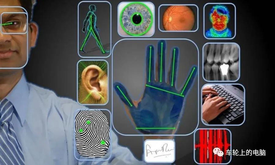
Face recognition, a type of biometric recognition technology, refers to the identification of individuals based on their inherent physiological characteristics (such as fingerprints, facial features, irises, palm prints, veins, etc.) or long-term behavioral traits (such as handwriting, voice, gait, etc.). Generally speaking, the convenience and security of this technology far exceed traditional identity verification methods like passwords and PINs. The mainstream biometric recognition technologies currently include fingerprint recognition, face recognition, iris recognition, voice recognition, vein recognition, and voiceprint recognition (see Figure 1).
Figure 1 Examples of Common Biometric Recognition Technologies[1]
The face is the most common and familiar biological feature in daily life. Face recognition technology is widely used in security, payment, attendance, finance, and other fields, significantly enhancing the safety and convenience of people’s lives. Compared to other biometric recognition technologies, face recognition can be widely applied due to the following advantages:
Unlike fingerprint recognition, which requires users to place their fingers on a fingerprint scanner, face recognition does not require contact with the human body; it directly collects facial image information through front-end devices like cameras.
The non-contact nature of face recognition provides users with a non-intrusive experience. First, face image collection does not require manual intervention and can be automatically collected without awareness; moreover, since the face is an exposed biological feature, collecting facial images is relatively easy for ordinary users to accept.
Well-developed and easily expandable hardware
Compared to fingerprint recognition or iris recognition, which require specific collection devices, a face recognition system only needs a camera and a computer, combined with relevant software algorithms, making it cost-effective. Given the widespread use of mobile and smart devices, it is also easy to expand.
The Past and Present of Face Recognition
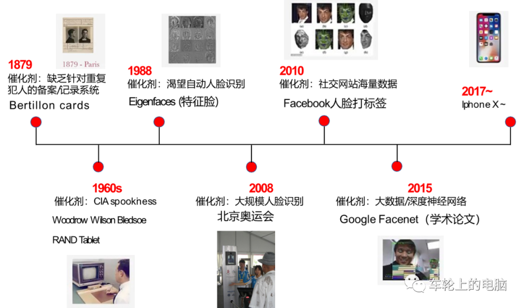
The use of facial features for identity verification dates back to the 1870s. A Parisian police officer named Alphonse Bertillon developed a method of “anthropometry” based on human features (including some facial characteristics). He believed that by the age of 20, the human skeleton would have basically formed. By recording multiple sets of data such as head length, head width, middle finger length, ear length, height, and sitting height, along with corresponding facial photographs, he aimed to compare and identify criminals. However, this entirely manual method was time-consuming and labor-intensive, with low accuracy, necessitating the urgent development of an automated high-precision face recognition system.
The research on truly automated face recognition systems began in the 1960s, and improved in the 1980s with advancements in computer technology and optical imaging technology. The 2008 Beijing Olympics introduced face recognition for rapid identity verification. With the accumulation of large-scale facial data (massive facial data tagging on platforms like Facebook) and the rapid development of deep learning technology, deep learning-based face recognition technology has gradually become mainstream in research and application.
In 2015, Google published a paper on FaceNet[3], achieving a high accuracy of 99.63% on the commonly used face recognition verification dataset LFW. In 2017, Apple released the iPhone X, which for the first time implemented facial unlocking on a mobile device, sparking a wave of research and application in face recognition technology.
Figure 2 Major Stages in the Development of Face Recognition Technology[2]
Understanding the Face Recognition Process
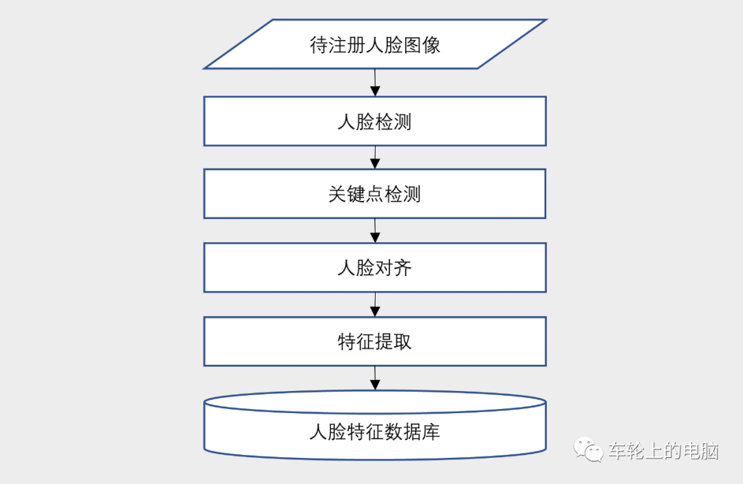
Everyone has probably used the facial unlock feature on their phone. During the first use of this feature, a facial registration process is required (Figure 3) to create a facial template, allowing for subsequent online facial recognition comparisons for login (Figure 4).
Figure 3 Facial Registration Process
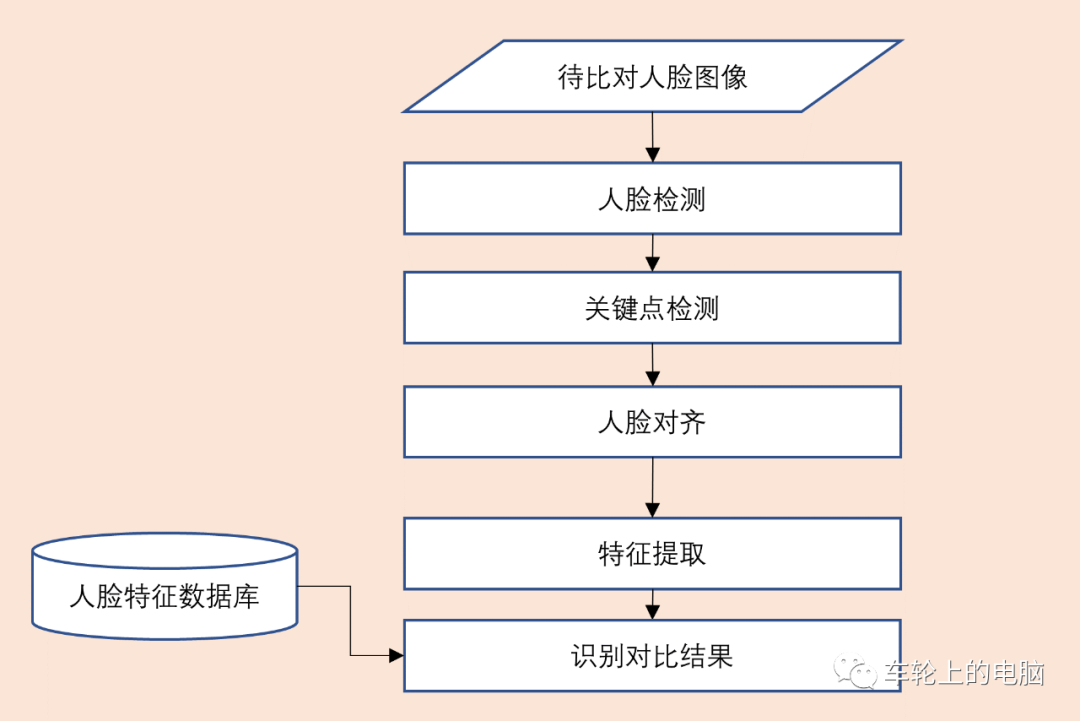
Figure 4 Face Recognition Process
There are generally three modes of face recognition: 1:1, 1:N, and M:N.
This mode is typically used for identity verification, which can be understood as proving “you are you”. For example, when taking a train/plane or applying for a bank card, it is usually necessary to verify that the person is indeed the one holding the ID.
This mode compares a facial image with all faces in a facial feature database one by one. It searches for similar images (where the similarity of facial comparisons exceeds a set threshold) in the facial database, effectively identifying “who you are.” Common scenarios include suspect tracking, community access control, and company attendance.
This mode compares two facial databases. For example, if facial database A has M faces and database B has N faces, to determine how many faces are the same between A and B, each of the M faces in database A must be compared with each of the N faces in database B, equivalent to adding M instances of 1:N comparisons.
From Figures 3 and 4, it can be seen that whether in the registration or recognition phase, the process generally includes several important steps: face detection, facial key point detection, face alignment, and facial feature extraction. This article will first introduce face detection technology.
Face detection refers to accurately locating the position and size of the face in a given facial image. Only by knowing where the face is in the image can subsequent facial-related tasks be carried out. Therefore, face detection is the foundational algorithm for facial-related algorithms and engineering implementation. Face detection can be considered a subset of object detection. Object detection (also known as general object detection) targets multiple categories, while face detection is binary classification, resulting in either face or non-face.
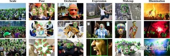
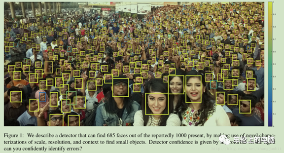
Theoretically, general object detection algorithms can be directly used for face detection by simply modifying the output categories. General object detection considers a broader range of objects, with more complex scenarios, shapes, backgrounds, and sizes than the single category of faces. Although face detection has a single category, it is not simple; challenges such as pose, lighting, occlusion (see Figure 5), and extremely small faces (see Figure 6) are all difficulties within face detection. Based on general object detection algorithms, face detection issues can be specifically optimized, such as anchor settings, background processing, and suppression of false detections.
Figure 5 Effects of Pose, Lighting, Occlusion, etc.[4]
Figure 6 Small Face Detection[5]
Before introducing specific detection algorithms, let’s first discuss commonly used face detection databases and evaluation metrics.
Common face detection databases include: FDDB[6] and WIDER FACE[4].
FDDB is one of the most authoritative face detection evaluation databases in the world, fully public, with a total of 2845 images and 5171 face annotations. It includes facial images with different poses, resolutions, rotations, and occlusions, as well as grayscale and color images. The images have a relatively small resolution, with all images having their longest edge scaled to 450 pixels, meaning all images are less than 450*450, and the minimum annotated face size is 20*20. The vast majority of images contain only one face.
It contains a total of 32203 images and 393703 face annotations, divided into training set (train)/validation set (val)/test set (test), accounting for 40%/10%/50% respectively. The dataset includes facial images of various scales, poses, occlusions, expressions, makeup, lighting, etc., with a high level of difficulty. The images generally have a higher resolution, with all images’ width scaled to 1024, and the minimum annotated face size is 10*10, consisting of color images; on average, there are 12.2 faces/image, with many small dense faces.
WIDER FACE does not publicly disclose the annotated results of the test set (GT: ground truth), requiring submissions for evaluation by the official organization, ensuring fairness and reliability, and the test set is large. Based on the detection rates of the EdgeBox method, the WIDER FACE evaluation set is divided into three difficulty levels: Easy, Medium, Hard. Algorithms can be evaluated across various task dimensions, such as the Hard level being very suitable for evaluating small faces.
02 Common Evaluation Metrics
The most commonly used evaluation metrics for binary classification problems are accuracy and recall:
-
Accuracy (Precision) represents how many of the predicted positive samples are actual positive samples;
-
Recall represents how many of the total positive samples are successfully predicted (predicted as positive).
To illustrate how to calculate accuracy and recall, let’s assume there are 100 positive samples and 100 negative samples in the test set, with 90 of the 100 positive samples correctly predicted as positive and 10 incorrectly predicted as negative; among the 100 negative samples, 80 are correctly predicted as negative and 20 are incorrectly predicted as positive:
-
TP (true positive) represents the number of positive samples correctly predicted as positive, so TP=90;
-
TN (true negative) represents the number of negative samples correctly predicted as negative, so TN=80;
-
FP (false positive) represents the number of negative samples incorrectly predicted as positive, so FP=20;
-
FN (false negative) represents the number of positive samples incorrectly predicted as negative, so FN=10.
With these four values, we can calculate:
-
Accuracy Precision = TP/(TP+FP)=90/(90+20)=0.818
-
Recall = TP/(TP+FN)=90/(90+10)=0.900
In the previously mentioned face detection, there are only two categories: face and background. To evaluate the performance of face detection algorithms using accuracy and recall, the detection framework must define what constitutes a correct detection. Generally, when the detection box and GT’s IOU (Intersection over Union) exceed a given threshold (e.g., 0.7), it is considered that the face has been correctly detected; based on this premise, statistics can be compiled according to binary classification.
Continuing with the previous example, suppose there are 100 faces in the actual test set, and the algorithm detects 95 face boxes, of which 90 meet the threshold requirement and are considered correct detections, while the remaining 5 are considered false detections. Then TP/TN/FP/FN can be calculated as follows:
-
TP: 90 out of 100 faces are correctly predicted, so TP=90;
-
TN: No background is output, so TN=0;
-
FP: Predicted as a face, but actually non-face, meaning there are 5 false detections, so FP=5;
-
FN: Positive samples that were not detected, meaning there are 10 missed detections, so FN=100-90=10.
With these four values, we can calculate:
-
Accuracy Precision = TP/(TP+FP)=90/(90+5)=0.947
-
Recall = TP/(TP+FN)=90/(90+10)=0.900
Based on different thresholds, many pairs of accuracy Precision and recall Recall can be obtained, leading to the generation of a PR curve, as shown in Figure 7.
Figure 7 PR Curve Example[4]
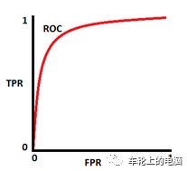
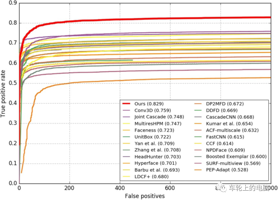
ROC curve is another metric for evaluating binary classification algorithms. The vertical axis represents the true positive rate (True Positive Rate, TPR=TP/(TP+FN)), and the horizontal axis represents the false positive rate (False Positive Rate, FPR=FP/(TN+FP)).
Similarly, many pairs of TPR and FPR can be obtained based on different thresholds, leading to the generation of an ROC curve (see Figure 8).
Figure 8 ROC Curve Example[29]
Next, we will specifically introduce face detection algorithms. We will divide the entire face detection algorithm into three stages: early algorithms, the AdaBoost framework, and deep learning frameworks.
Early algorithms used template matching techniques, matching a facial template image with various positions in the detected image to determine whether a face exists at that position; the AdaBoost framework is represented by a face detection algorithm designed by Viola and Jones in 2001[7]. It uses Haar-like features and a cascade of AdaBoost classifiers, achieving a two-order of magnitude speed increase compared to previous methods while maintaining good accuracy, commonly referred to as the VJ framework. The VJ framework is the first milestone achievement in the history of face detection, laying the foundation for the AdaBoost-based object detection framework. Before the advent of deep learning methods, industry solutions were mainly based on the VJ algorithm; with the success of convolutional neural networks in image classification, they were quickly applied to face detection, greatly surpassing previous algorithms in accuracy and gradually becoming the mainstream in research and application.
03 Face Detection Based on AdaBoost Classifier
The classic flowchart of the face detection algorithm is as follows:
Figure 9 Classic Face Detection Algorithm Flowchart
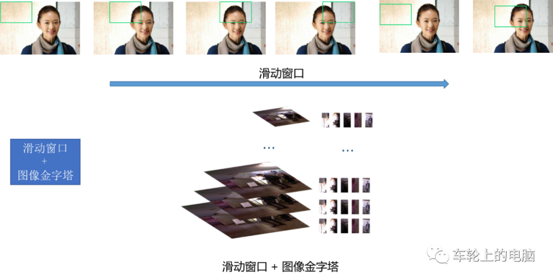
Faces may appear in any position in the image, so a fixed-size window is used to scan the image from top to bottom and left to right with a certain step size, known as the sliding window technique. Additionally, to detect faces of different sizes, the image is scaled to construct an image pyramid, and the sliding window technique is applied to each scaled image.
Figure 10 Sliding Window + Image Pyramid (Image from the Internet)
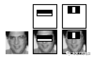
After obtaining the image sub-windows, corresponding feature descriptors are extracted. The commonly used feature descriptor in actual detection is the Haar-like feature proposed by Viola and Jones in 2001[7]. Figure 11 is a schematic diagram of Haar-like features. Haar-like features are the sum of pixel values within the white rectangular box, minus the sum of pixel values within the black area. These features capture information about edges and variations in the image, representing image changes in various directions. The facial features have distinct brightness information, which aligns well with the characteristics of Haar-like features.
Figure 11 Schematic Diagram of Basic Haar-like Features[7]
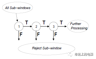
Due to the use of sliding window scanning technology and the need to repeatedly scale and scan the image, the number of images obtained is very high, and the vast majority of windows are backgrounds, meaning faces are a sparse event. If non-face windows can be quickly excluded, it will greatly improve the efficiency of object detection. Therefore, a cascade classifier like AdaBoost is used for face detection. The essence of this idea is to use simple weak classifiers to quickly eliminate a large number of non-face windows in the early stages while ensuring a high recall rate; ultimately, windows passing through all weak classifiers are considered to contain faces. Figure 12 is a schematic diagram of the classifier cascade judgment:
Figure 12 Example of AdaBoost Cascade Classifier[7]: Three Cobbler’s Work Together to Match One Zhuge Liang
04 Face Detection Based on Deep Learning
After the success of convolutional neural networks in image classification, they were quickly applied to face detection, surpassing the previous AdaBoost framework in accuracy. Furthermore, using a sliding window for face detection requires a large amount of computation, making it difficult to achieve real-time performance; therefore, various methods are employed to optimize this issue.
Cascade CNN[8] draws inspiration from the AdaBoost face detector concept, which also includes multiple classifiers organized in a cascade structure. The difference is that Cascade CNN uses convolutional networks as the classifier at each level. First, a small network called 12-net is used to search for dense candidate face regions in the input image, where the detection region is 12×12, and the search step is 4 pixels, quickly eliminating 90% of non-face areas. The remaining detection windows are sent to the 12-calibration-net to adjust their size and position. Non-maximum suppression (NMS) is then applied to merge highly overlapping detection windows, and the remaining candidate detection windows will be normalized to 24×24 and sent to the 24-net. The 24-net will further filter the remaining nearly 90% of detection windows. As in the previous process, the 24-calibration-net corrects the detection window, and NMS is applied again to further reduce the number of detection windows. The remaining candidate detection windows are then normalized to 48×48 and sent to the 48-net for classification to obtain further filtered face candidate windows. Finally, NMS is used for window merging, and the 48-calibration-net corrects the detection window as the final output (see algorithm structure in Figure 13).
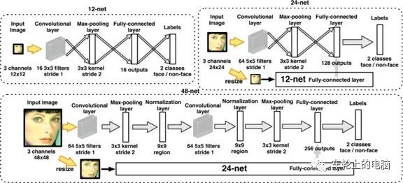 Figure 13 Cascade CNN[8] Algorithm Pipeline
Some papers suggest that adding auxiliary tasks for multi-task learning in face detection can improve detection performance. MTCNN[9] incorporates facial key point detection into the face detection task, improving detection performance through the collaboration of the two tasks. Like Cascade CNN, it is also based on a cascade framework. MTCNN can be divided into three parts: P-Net, R-Net, and O-Net (see Figure 14). MTCNN utilizes a shallow network P-Net to rapidly generate candidate windows, a slightly more complex network R-Net to eliminate a large number of non-face windows, and finally a more powerful network O-Net to further improve results and jointly output facial key point locations. Unlike the 12-net of Cascade CNN[8], which requires dense window sampling across the entire image for classification, the P-Net of MTCNN is a fully convolutional network (FCN), which allows for input of images of any size and replaces sliding window operations with convolution operations, significantly improving detection efficiency.
Figure 13 Cascade CNN[8] Algorithm Pipeline
Some papers suggest that adding auxiliary tasks for multi-task learning in face detection can improve detection performance. MTCNN[9] incorporates facial key point detection into the face detection task, improving detection performance through the collaboration of the two tasks. Like Cascade CNN, it is also based on a cascade framework. MTCNN can be divided into three parts: P-Net, R-Net, and O-Net (see Figure 14). MTCNN utilizes a shallow network P-Net to rapidly generate candidate windows, a slightly more complex network R-Net to eliminate a large number of non-face windows, and finally a more powerful network O-Net to further improve results and jointly output facial key point locations. Unlike the 12-net of Cascade CNN[8], which requires dense window sampling across the entire image for classification, the P-Net of MTCNN is a fully convolutional network (FCN), which allows for input of images of any size and replaces sliding window operations with convolution operations, significantly improving detection efficiency.
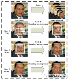 Figure 14 MTCNN Algorithm Pipeline[9]
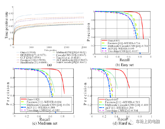
The MTCNN algorithm achieved state-of-the-art results on FDDB and WIDER FACE (see Figure 15). For details, please refer to paper[9].
Figure 15 MTCNN[9] Evaluation Results, (a) FDDB; (b-d) 3 subsets of WIDER FACE.
In practical applications, a trade-off between real-time performance and accuracy needs to be sought, as networks with high accuracy often involve substantial computation, resulting in slower speeds.
FaceBoxes[10] is a lightweight face detector proposed by Professor Li Ziqing’s team at the Chinese Academy of Sciences in 2017, aiming to achieve real-time face detection on CPUs, as the article title suggests. Figure 16 presents the corresponding algorithm pipeline. It addresses the issues present in MTCNN: 1) Detection speed is affected by the number of faces; 2) Multi-stage training complicates the process; 3) Speed remains slow, and proposes the following innovations:
Figure 14 MTCNN Algorithm Pipeline[9]
The MTCNN algorithm achieved state-of-the-art results on FDDB and WIDER FACE (see Figure 15). For details, please refer to paper[9].
Figure 15 MTCNN[9] Evaluation Results, (a) FDDB; (b-d) 3 subsets of WIDER FACE.
In practical applications, a trade-off between real-time performance and accuracy needs to be sought, as networks with high accuracy often involve substantial computation, resulting in slower speeds.
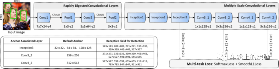
FaceBoxes[10] is a lightweight face detector proposed by Professor Li Ziqing’s team at the Chinese Academy of Sciences in 2017, aiming to achieve real-time face detection on CPUs, as the article title suggests. Figure 16 presents the corresponding algorithm pipeline. It addresses the issues present in MTCNN: 1) Detection speed is affected by the number of faces; 2) Multi-stage training complicates the process; 3) Speed remains slow, and proposes the following innovations:
-
Using the RDCL (Rapidly Digested Convolutional Layers) module to quickly reduce the feature map size, ensuring detection speed: by appropriately sizing convolution kernels to rapidly shrink the input space, reducing the number of output channels, FaceBoxes achieves real-time speed on CPU devices;
-
The MSCL (Multiple Scale Convolutional Layers) module uses multi-scale feature maps for predictions, handling faces at different scales;
-
Using an anchor densification strategy to improve the recall rate of small faces.
Figure 16 FaceBoxes[10] Algorithm Pipeline
Inputting VGA resolution images, the speed on a single CPU core ([email protected]) is 20FPS, and on GPU (Titan X (Pascal)) it is 125FPS. The method also achieved state-of-the-art results on FDDB (see Figure 17).
Figure 17 FaceBoxes[10] Experimental Results on FDDB
In 2019, Google released a lightweight and high-performance face detector specifically designed for mobile GPU inference—an ultra-millisecond face detection algorithm called BlazeFace[11]. It can run at speeds of 200-1000+ FPS on flagship devices. This ultra-real-time performance allows BlazeFace to be applied in any real-world application with high performance requirements, such as on mobile phones. The main innovations of this method are:
-
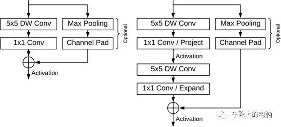
Inspired by MobileNet, the extremely lightweight feature extraction network BlazeBlock was proposed. Specifically, it uses 5*5 convolution kernels instead of 3*3 convolution kernels, which does not incur significant overhead but increases the receptive field. Under front-facing cameras, the scale of faces changes minimally, allowing for a more lightweight feature extraction definition, with input images at 128*128, containing 5 BlazeBlocks and 6 double BlazeBlocks (see Figure 18).
Figure 18 Structure Diagram of BlazeBlock and Double BlazeBlock [11]
-
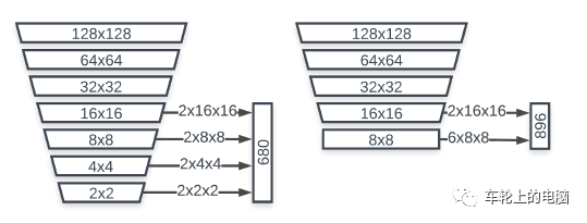
Optimized anchor mechanism, stopping down-sampling at the 8*8 feature map size (see Figure 19), replacing each pixel in 8*8, 4*4, and 2*2 resolutions with 6 anchors at 8*8. Given the limited aspect ratio variation of faces, fixing the anchors at 1:1 is sufficient for accurate face detection.
Figure 19 Anchor Calculation: SSD (left) vs. BlazeFace [11]
BlazeFace emphasizes the acceleration of detection algorithms in real applications on mobile terminals, thus it does not compare with state-of-the-art algorithms on public datasets in terms of accuracy, but only compares with MobileNetV2-SSD on Google’s private dataset. Figure 20 shows the comparison results, indicating higher accuracy than MobileNetV2-SSD, with speed on the iPhone XS dropping from 2.1ms to 0.6ms. Additionally, BlazeFace achieves significant speed improvements on various mobile phones.
Figure 20 Detection Performance and Inference Time [11]
Face recognition technology has developed significantly over the years, becoming rich in content and widely applied. This article has explained the history of face recognition, the technical process, and highlighted the face detection algorithms, hoping to help everyone understand and recognize the face recognition functionality we have become accustomed to. Next time, we will continue to explain another key technology in face recognition—facial key point detection algorithms. See you next time!
References:
[1] Science Popularization Article丨Biometric Recognition: Confirmed “Palm Print” to Find the Right Person
http://www.ioa.cas.cn/kxchb/kpzp/kpwz/202112/t20211222_6325383.html
[2] Adjabi, Insaf, et al. “Past, present, and future of face recognition: A review.” Electronics 9.8 (2020): 1188.
[3] Schroff, Florian, Dmitry Kalenichenko, and James Philbin. “Facenet: A unified embedding for face recognition and clustering.” Proceedings of the IEEE conference on computer vision and pattern recognition. 2015.
[4] http://shuoyang1213.me/WIDERFACE/
[5] Hu, Peiyun, and Deva Ramanan. “Finding tiny faces.” Proceedings of the IEEE conference on computer vision and pattern recognition. 2017.
[6] http://vis-www.cs.umass.edu/fddb/index.html
[7] Viola P, Jones M. Rapid object detection using a boosted cascade of simple features[C]//Proceedings of the 2001 IEEE computer society conference on computer vision and pattern recognition. CVPR 2001. IEEE, 2001, 1: I-I.
[8] Li, Haoxiang, et al. “A convolutional neural network cascade for face detection.” Proceedings of the IEEE conference on computer vision and pattern recognition. 2015.
[9] Zhang K, Zhang Z, Li Z, et al. Joint face detection and alignment using multitask cascaded convolutional networks[J]. IEEE Signal Processing Letters, 2016, 23(10): 1499-1503.
[10] Zhang S, Zhu X, Lei Z, et al. Faceboxes: A CPU real-time face detector with high accuracy[C]//2017 IEEE International Joint Conference on Biometrics (IJCB). IEEE, 2017: 1-9.
[11] Bazarevsky, Valentin, et al. “Blazeface: Sub-millisecond neural face detection on mobile gpus.” arXiv preprint arXiv:1907.05047 (2019).
[12] https://www.52cv.net/?p=1006
[13] https://www.nist.gov/programs-projects/face-recognition-grand-challenge-frgc
[14] https://www.cs.cmu.edu/~deva/papers/face/face-cvpr12.pdf
[15] https://www.tugraz.at/institute/icg/research/team-bischof/lrs/downloads/aflw/
[16] https://ieeexplore.ieee.org/document/6751298
[17] https://ibug.doc.ic.ac.uk/resources/300-W/
[18] Belhumeur, P., Jacobs, D., Kriegman, D., Kumar, N.. ‘Localizing parts of faces using a consensus of exemplars’. In Computer Vision and Pattern Recognition, CVPR. (2011).
[19] X. Zhu, D. Ramanan. ‘Face detection, pose estimation and landmark localization in the wild’, Computer Vision and Pattern Recognition (CVPR) Providence, Rhode Island, June 2012.
[20] Vuong Le, Jonathan Brandt, Zhe Lin, Lubomir Boudev, Thomas S. Huang. ‘Interactive Facial Feature Localization’, ECCV2012.
[21] Messer, K., Matas, J., Kittler, J., Luettin, J., Maitre, G. ‘Xm2vtsdb: The extended m2vts database’. In: 2nd international conference on audio and video-based biometric person authentication. Volume 964. (1999).
[22] https://wywu.github.io/projects/LAB/WFLW.html
[23] https://facial-landmarks-localization-challenge.github.io/
[24] T.F. Cootes, C.J. Taylor, D.H. Cooper, et al. Active Shape Models-Their Training and Application[J]. Computer Vision and Image Understanding, 1995, 61(1):38-59.
[25] G. J. Edwards, T. F. Cootes, C. J. Taylor. Face recognition using active appearance models[J]. Computer Vision—Eccv, 1998, 1407(6):581-595.
[26] Dollár P, Welinder P, Perona P. Cascaded pose regression[J]. IEEE, 2010, 238(6):1078-1085.
[27] Sun Y, Wang X, Tang X. Deep convolutional network cascade for facial point detection, CVPR. 2013: 3476-3483.
[28] Zhang Z, Luo P, Loy C C, et al. Facial landmark detection by deep multi-task learning, European conference on computer vision. Springer, Cham, 2014: 94-108.
[29] https://towardsdatascience.com/understanding-auc-roc-curve-68b2303cc9c5
[30] O. Jesorsky, K. J. Kirchberg, and R. Frischholz. Robust face detection using the hausdorff distance. In Proc. AVBPA, 2001.
[31] P. N. Belhumeur, D. W. Jacobs, D. J. Kriegman, and N. Kumar. Localizing parts of faces using a consensus of exemplars. In Proc. CVPR, 2011.