
1. R-CNN: Rich feature hierarchies for accurate object detection and semantic segmentation
Technical route: selective search + CNN + SVMs
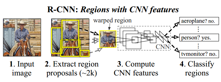
Step 1: Candidate box extraction (selective search)
Training: Given an image, use the selective search method to extract 2000 candidate boxes. Since the sizes of the candidate boxes vary, considering the CNN’s requirement for uniform input size, all 2000 candidate boxes are resized to a resolution of 227*227 (to avoid severe distortion, some techniques can be applied to reduce image distortion).
Testing: Given an image, use the selective search method to extract 2000 candidate boxes. Since the sizes of the candidate boxes vary, considering the CNN’s requirement for uniform input size, all 2000 candidate boxes are resized to a resolution of 227*227 (to avoid severe distortion, some techniques can be applied to reduce image distortion).
Step 2: Feature extraction (CNN)
Training: The CNN model for feature extraction needs to be pre-trained. During CNN training, the labeling requirements for training data are relatively loose; that is, when the proposal extracted by the SS method only includes part of the target area, we still label this proposal as a specific object category. The main reason for this is that CNN training requires a large amount of data. If the labeling requirements are extremely strict (i.e., only completely containing the target area and the area not belonging to the target cannot exceed a small threshold), then the number of samples for CNN training will be very small. Therefore, the CNN model trained under loose labeling conditions can only be used for feature extraction.
Testing: After obtaining the uniformly sized 227*227 proposals, they are input into the trained CNN model, and the output of the last fully connected layer — a 4096*1 dimensional vector is used as the final test feature.
Step 3: Classifier (SVMs)
Training: For all proposals, strict labeling is performed (it can be understood that a candidate box is labeled as a target only when it completely contains the ground truth area and does not exceed, for example, 5% of the candidate box area that does not belong to the ground truth area; otherwise, it is considered background), and then all proposals are processed through CNN to obtain features, and the new labeling results are input into the SVM classifier for training to obtain the classifier prediction model.
Testing: For a test image, the 2000 proposals extracted undergo CNN feature extraction and are input into the SVM classifier prediction model, which can provide specific category score results.
Result generation: After obtaining the SVM scores for all proposals, some proposals with lower scores are removed, and among the remaining proposals, there will be cases of overlapping candidate boxes. Non-maximum suppression technology is used to find the candidate box that best represents the final detection result among the intersecting boxes (for more information on non-maximum suppression methods, refer to: http://blog.csdn.net/pb09013037/article/details/45477591)
R-CNN requires performing a forward CNN for each proposal extracted by SS for feature extraction, so the computational load is very high and cannot be performed in real-time. Additionally, due to the existence of fully connected layers, it is necessary to ensure that the input proposals are resized to the same scale, which can cause some degree of image distortion and affect the final results.
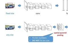
2. SPP-Net: Spatial Pyramid Pooling in Deep Convolutional Networks for Visual Recognition
The comparison of the traditional CNN and SPP-Net processes is shown in the figure below (from http://www.image-net.org/challenges/LSVRC/2014/slides/sppnet_ilsvrc2014.pdf)
SPP-net has the following characteristics:
1. In traditional CNN networks, the convolutional layer does not have special requirements on the input image size, but the fully connected layer requires the input image to have a uniform size. Therefore, in R-CNN, for the proposals of different sizes proposed by the selective search method, it is necessary to first use Crop or Warp operations to cut the proposal area to a uniform size and then use CNN to extract proposal features. In contrast, SPP-net adds a spatial pyramid pooling (SPP) layer between the last convolutional layer and the subsequent fully connected layer, thereby avoiding the need to Crop or Warp proposals. In summary, the SPP layer is suitable for input images of different sizes; through the SPP layer, the features of the last convolutional layer are pooled to produce a fixed-size feature map, which can match the subsequent fully connected layer.
2. Since SPP-net supports input images of different sizes, the image features extracted by SPP-net have better scale invariance, reducing the likelihood of overfitting during the training process.
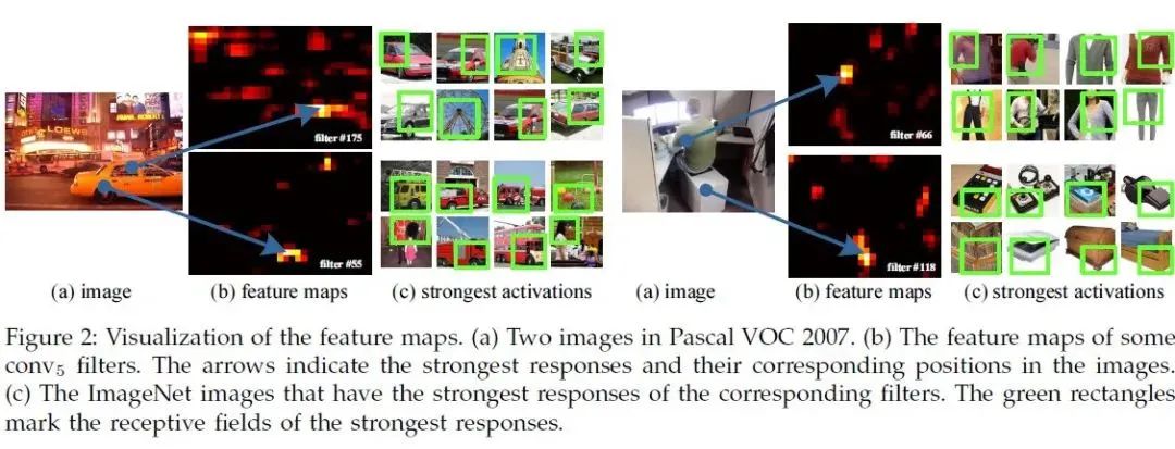
3. R-CNN requires performing a forward CNN feature extraction for each proposal in each image during training and testing. If there are 2000 proposals, it requires 2000 forward CNN feature extractions. However, SPP-net only needs to perform one forward CNN feature extraction for the entire image to obtain the feature map of the last convolutional layer, and then use the SPP layer to obtain the corresponding features for each proposal based on spatial correspondence. The speed of SPP-net can be 24 to 102 times faster than R-CNN, and its accuracy is higher than R-CNN (the figure below is from the original SPP-net paper; it can be seen that there are 5 convolutional layers before the SPP-layer in SPP-net, and the output features of the 5th convolutional layer can correspond to the original image, for example, the left bottom wheel of the first image is shown as the activation area of “^” in its conv5 image; thus, based on this feature, SPP-net only needs to perform one forward convolution for the entire image, then use SPP-net to extract the corresponding proposal features).
SPP-Layer principle:
In RNN, after conv5 is pool5; in SPP-net, the SPP-layer replaces the original pool5; its goal is to ensure that the feature vector length obtained after passing through the SPP-Layer is the same for input images of different sizes. The principle is shown in the figure below
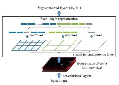
SPP is similar to pyramid pooling; we first determine the final pooling feature map size, such as 4*4 bins, 3*3 bins, 2*2 bins, and 1*1 bins. We know the feature map size output from conv5 (for example, 256 feature maps of 13*13). For a 13*13 feature map, we can obtain the output result through spatial pyramid pooling (SPP): when window=ceil(13/4)=4, stride=floor(13/4)=3, we can obtain 4*4 bins; when window=ceil(13/3)=5, stride=floor(13/3)=4, we can obtain 3*3 bins; when window=ceil(13/2)=7, stride=floor(13/2)=6, we can obtain 2*2 bins; when window=ceil(13/1)=13, stride=floor(13/1)=13, we can obtain 1*1 bins. Therefore, the output after the SPP-layer is 256*(4*4+3*3+2*2+1*1)=256*30 length vector. It is not difficult to see that the key to SPP lies in calculating the pooling window and pool stride sizes corresponding to different resolution bins in spatial pyramid pooling based on the width and height of the feature map output from conv5 and the width and height of the SPP target output bins.
The original author used two different methods during training: 1. Training SPP-net with images of the same size. 2. Training SPP-net with images of different sizes. Experimental results show that using images of different sizes for training yields better results for SPP-Net.
SPP-Net + SVM training:
Using selective search, a series of proposals can be extracted. Since SPP-Net has been trained, we first input the entire image into SPP-Net to obtain the output of conv5. Next, unlike R-CNN, the new method does not need to Crop or Warp different sized proposals; instead, it directly computes the mapping output of the proposal in the entire image based on the relative position relationship of the proposals. Thus, for 2000 proposals, we actually perform one forward pass from conv1 to conv5 and then perform 2000 sets of mapping of conv5 feature maps, and through the SPP-Layer, we can obtain 2000 sets of length-equal SPP-Layer output vectors, which can then be fed into fully connected layers to generate the final convolutional neural network features for the 2000 proposals. The process is similar to R-CNN; during SVM training, all proposals undergo strict labeling (it can be understood that a candidate box is labeled as a target only when it completely contains the ground truth area and does not exceed, for example, 5% of the candidate box area that does not belong to the ground truth area; otherwise, it is considered background), and then all proposals processed through CNN to obtain features and the new labeling results are input into the SVM classifier for training to obtain the classifier prediction model.
Of course, if SVM training is considered cumbersome, one can directly add a softmax layer after SPP-Net and use good labeling results to train the parameters of the final softmax layer.
3. Fast-R-CNN
Based on the ideas of R-CNN and SPP-Net, RBG proposed the Fast-R-CNN algorithm. If VGG16 is chosen for feature extraction, during the training phase, the speed of Fast-R-CNN can be improved by 9 times compared to RCNN and 3 times compared to SPP-Net; during the testing phase, the speed of Fast-R-CNN can be improved by 213 times compared to RCNN and 10 times compared to SPP-Net.
Disadvantages of R-CNN and SPP-Net:
1. The training process of R-CNN and SPP-Net is similar, conducted in multiple stages, making the implementation process complex. Both methods first use the Selective Search method to extract proposals, then use CNN for feature extraction, and finally train the classifier based on SVMs. Additionally, further learning of the bounding box for the detection target can be performed.
2. R-CNN and SPP-Net have high time and space costs. SPP-Net only requires one forward CNN computation for the entire image during the feature extraction phase, and then calculates the corresponding CNN features for each proposal through spatial mapping; in contrast, R-CNN requires one forward CNN computation for each proposal during the feature extraction phase. Considering the large number of proposals (~2000), the time cost for feature extraction in R-CNN is very high. The features used for training the SVM classifiers in R-CNN and SPP-Net need to be stored on disk in advance; considering the total amount of CNN features for 2000 proposals is relatively large, this incurs a high space cost.
3. The detection speed of R-CNN is very slow. R-CNN requires one forward CNN computation for each proposal during the feature extraction phase, and if using VGG for feature extraction, it takes 47 seconds to process all proposals for one image.
4. The training of the feature extraction CNN and the training of the SVM classifier are sequential in time, and their training methods are independent. Therefore, the training loss of the SVM cannot update the parameters of the convolutional layers before the SPP-Layer. Thus, even if a deeper CNN is used for feature extraction, it cannot guarantee that the accuracy of the SVM classifier will necessarily improve.
Highlights of Fast-R-CNN:
1. Fast-R-CNN achieves better detection results than R-CNN and SPP-Net.
2. The training method is simple, based on multi-task loss, eliminating the need for SVM training for the classifier.
3. Fast-R-CNN can update the network parameters of all layers (the ROI Layer will no longer require the use of the SVM classifier, allowing for end-to-end training of the entire network).
4. There is no need to cache features to disk.
The architecture of Fast-R-CNN is shown in the figure below (https://github.com/rbgirshick/fast-rcnn/blob/master/models/VGG16/train.prototxt; you can refer to this link to understand the network model): input an image and a series of proposals generated by the Selective Search method, through a series of convolutional layers and pooling layers to generate feature maps, then use the RoI (region of interest) layer to process the feature map obtained from the last convolutional layer to generate a fixed-length feature vector roi_pool5 for each proposal. The output roi_pool5 from the RoI layer is then input into fully connected layers to produce the final features for multi-task learning and compute multi-task loss. The fully connected output includes two branches: 1. SoftMax Loss: calculating the classification loss function for K+1 classes, where K represents K object categories and 1 represents background; 2. Regression Loss: the coordinates of the four corners of the bounding box corresponding to the classification results of K+1. Finally, all results are processed through non-maximum suppression to produce the final object detection and recognition results.
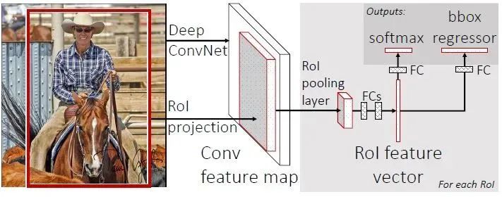
3.1 RoI Pooling Layer
In fact, the RoI Pooling Layer is a simplified version of the SPP-Layer. The SPP-Layer is a spatial pyramid pooling layer that includes different scales; the RoI Layer only contains one scale, as described in the paper, 7*7. Thus, for the input of the RoI Layer (r,c,h,w), the RoI Layer first generates 7*7 blocks of size r*c*(h/7)*(w/7), and then uses Max-Pool to find the maximum value of each block, resulting in an output of r*c*7*7 for the RoI Layer.
ROIs Pooling, as the name suggests, is a type of pooling layer, specifically for pooling RoIs, characterized by fixed output feature map sizes despite variable input feature map sizes.
What is an ROI? ROI stands for Region of Interest, referring to the “box on the feature map”; 1) in Fast RCNN, the RoI refers to the “candidate box” obtained after the completion of Selective Search mapped on the feature map, as shown in the figure below; 2) in Faster RCNN, the candidate boxes are generated by RPN, and then each “candidate box” is mapped to the feature map, obtaining RoIs.
3.2 Pre-trained Network Initialization
RBG reused the VGG model trained on ImageNet to initialize all layers before the RoI Layer in Fast-R-CNN. The overall network structure of Fast R-CNN can be summarized as follows: 13 convolution layers + 4 pooling layers + RoI layer + 2 fc layers + two parallel layers (i.e., SoftmaxLoss layer and SmoothL1Loss layer). In Fast R-CNN, the original 5th pooling layer of VGG16 is replaced by the new ROI layer.
3.3 Finetuning for Detection
3.3.1 Fast R-CNN employs some tricks during the network training phase, where each minibatch consists of R proposals (R=128) extracted from N images (N=2). This construction method for the minibatch is 64 times faster than constructing from 128 different images. Although the speed of minibatch construction is accelerated, it also slows down convergence to some extent. In addition, Fast R-CNN discards the previous SVM training classifier method and instead opts for joint training of the softmax classifier and bounding-box regressors to update all layer parameters of the CNN network. Note: When selecting 128 proposals from 2 images, it is crucial to ensure at least 25% of positive samples (proposals with IoU exceeding 0.5 with ground truth); the rest can all be considered background. During the training of the network model, no other forms of data augmentation operations are required.
3.3.2 Multi-task loss: Fast R-CNN includes two sub-layers of equal level, one for classification and the other for regression. The softmax loss corresponds to classification, while the smooth L1 Loss corresponds to regression. The weight ratio of the two losses is 1:1.
3.3.3 SGD hyper-parameters: The parameters for the fc layers used for softmax classification tasks and bounding-box regression are initialized using a Gaussian distribution with a standard deviation between 0.01 and 0.001.
3.4 Truncated SVD for Rapid Detection
In the detection phase, RBG uses truncated SVD to optimize larger FC layers, thereby accelerating detection speed when the number of RoIs is large.
Fast-R-CNN Experimental Conclusions:
1. The multi-task loss training method can improve algorithm accuracy.
2. Training Fast R-CNN with multi-scale images compared to single-scale images shows little improvement in mAP, but incurs significantly higher time costs. Therefore, considering training time and mAP, the author recommends using single-scale images for training Fast R-CNN directly.
3. The more images used for training, the higher the accuracy of the trained model.
4. The softmax loss training method yields slightly better results than SVM training, thus it cannot be proven that softmax loss is always superior to SVM; however, it simplifies the training process, eliminating the need for stepwise model training.
5. Proposals are not necessarily better when more are extracted; too many proposals can lead to a decrease in mAP.
4. Faster-R-CNN: Towards Real-Time Object Detection with Region Proposal Networks
In the previously introduced Fast-R-CNN, the first step requires the use of the Selective Search method to extract proposals from the image. Based on CPU implementation, Selective Search takes about 2 seconds to extract all proposals from an image. Excluding the proposal extraction time, Fast-R-CNN can perform real-time object detection. However, from an end-to-end perspective, the proposal extraction clearly becomes a bottleneck affecting the performance of the end-to-end algorithm. The latest EdgeBoxes algorithm, while improving the accuracy and efficiency of candidate box extraction to some extent, still takes 0.2 seconds to process a single image. Therefore, Ren Shaoqing proposed a new Faster-R-CNN algorithm, which introduces the RPN network (Region Proposal Network) for proposal extraction. The RPN network is a fully convolutional neural network that can extract proposals by sharing convolutional layer features; it only takes 10ms to extract a proposal from an image.
The Faster-R-CNN algorithm consists of two main modules: 1. The RPN candidate box extraction module 2. The Fast R-CNN detection module. Here, RPN is a fully convolutional neural network used to extract candidate boxes; Fast R-CNN detects and recognizes targets in the proposals extracted by RPN.

4.1 Region Proposal Network (RPN)
The input of the RPN network can be an image of any size (but it still has a minimum resolution requirement, for example, VGG is 228*228). If using VGG16 for feature extraction, the RPN network can be represented as VGG16+RPN.
VGG16: Refer to https://github.com/rbgirshick/py-faster-rcnn/blob/master/models/pascal_voc/VGG16/faster_rcnn_end2end/train.prototxt to see that the part of VGG16 used for feature extraction consists of 13 convolution layers (conv1_1—->conv5.3), excluding pool5 and the network structure after pool5.
RPN: RPN is a network that the author focuses on introducing, as shown in the figure below. The implementation method of RPN: on the convolution feature map of conv5-3, a sliding window of size n*n (the author chose n=3, i.e., a 3*3 sliding window) generates a fully connected feature of length 256 (corresponding to the ZF network) or 512 (corresponding to the VGG network). Then, after this 256 or 512 dimensional feature, two branches of fully connected layers are produced: 1. reg-layer, used to predict the coordinates x, y of the proposal’s center anchor point and its width and height w, h; 2. cls-layer, used to determine whether the proposal is foreground or background. The sliding window processing method ensures that the reg-layer and cls-layer are associated with the entire feature space of conv5-3. In fact, the author introduces the RPN layer implementation using fully connected layers to help us understand the process, but in practice, the author used convolutional layers to implement the function of fully connected layers. My personal understanding is that fully connected layers are just a special case of convolutional layers; if producing 256 or 512 dimensional fc features, they can be implemented using convolution layers with Num_out=256 or 512, kernel_size=3*3, stride=1 to map from conv5-3 to the first fully connected feature. Then, two layers with Num_out of 2*9=18 and 4*9=36, kernel_size=1*1, stride=1 are used to map features from the previous layer to the two branches of cls-layer and reg-layer. Note: Here, 2*9 indicates that the cls-layer classification results include two categories: foreground and background, while 4*9 indicates the four parameters of a proposal’s center point coordinates x, y and width, height w, h. Using convolution to implement fully connected processing does not reduce the number of parameters, but allows for more flexible input image sizes. In the RPN network, we need to understand the concept of anchors, the calculation method of loss functions, and the specific details of generating RPN layer training data.

Anchors: Literally understood as anchor points, located at the center of the previously mentioned n*n sliding window. For a sliding window, we can simultaneously predict multiple proposals, assuming there are k. The k proposals correspond to k reference boxes, each of which can be uniquely determined by a scale, an aspect_ratio, and the anchor point in the sliding window. Therefore, when we talk about an anchor later, understand it as an anchor box or reference box. The author defines k=9 in the paper, i.e., 3 scales and 3 aspect ratios determine the 9 reference boxes corresponding to the current sliding window position. The outputs of 4*k for the reg-layer and 2*k for the cls-layer score outputs. For a feature map of size W*H, there will be W*H*k anchor points. All anchors exhibit scale invariance.
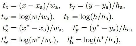
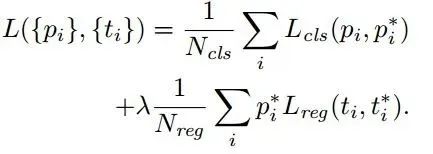
Loss functions: Before calculating the loss value, the author sets the labeling method for anchors. Positive sample labeling rules: 1. If the anchor’s corresponding reference box has the maximum IoU with the ground truth, it is labeled as a positive sample; 2. If the anchor’s corresponding reference box has IoU>0.7 with the ground truth, it is labeled as a positive sample. In fact, using the second rule can generally find enough positive samples, but for some extreme cases, such as when all anchors’ corresponding reference boxes have IoU not greater than 0.7, the first rule can be applied. Negative sample labeling rules: if the anchor’s corresponding reference box has IoU<0.3 with the ground truth, it is labeled as a negative sample. The rest, which are neither positive nor negative samples, are not used for final training. The loss for training RPN consists of classification loss (i.e., softmax loss) and regression loss (i.e., L1 loss) weighted accordingly. The calculation of softmax loss requires the ground truth labeling results and predicted results corresponding to anchors, while the calculation of regression loss needs three sets of information: 1. The predicted box, i.e., the coordinates x,y and width, height w,h of the proposal predicted by the RPN network; 2. The anchor reference box: the previously mentioned 9 anchors corresponding to 9 different scales and aspect ratios, each reference box having a center point position x_a,y_a and width, height w_a,h_a; 3. Ground truth: the labeled box also corresponds to a center point position x*,y* and width, height w*. Therefore, the calculation of regression loss and total loss is as follows:
RPN training settings: During RPN training, a mini-batch consists of 256 proposals randomly selected from a single image, maintaining a ratio of positive to negative samples of 1:1. If there are not enough positive samples (128), more negative samples are used to meet the requirement of having 256 proposals for training; conversely, if there are too many positive samples, some negative samples can be discarded. When training RPN, the shared layers’ parameters with VGG can directly copy parameters obtained from the ImageNet-trained model; the remaining layers’ parameters are initialized using a Gaussian distribution with a standard deviation of 0.01.
4.2 RPN and Faster-R-CNN Feature Sharing
After RPN extracts proposals, the author opts to use Fast-R-CNN to achieve final target detection and recognition. RPN and Fast-R-CNN share 13 convolutional layers of VGG, so it is not wise to train these two networks completely in isolation. The author adopts an alternating training phase with shared convolutional layer features:
Alternating training: Step 1: Train RPN; Step 2: Train Fast R-CNN using proposals obtained from RPN; Step 3: Initialize the shared convolutional layers in RPN using the parameters from Fast R-CNN. This process iterates through Steps 1, 2, and 3 until training is complete. The method used in the paper follows this training approach; note: during the first iteration, the RPN and Fast-R-CNN shared convolutional layer parameters are initialized using the model obtained from ImageNet; from the second iteration onward, the shared convolutional layer parameters in RPN are initialized using the shared convolutional layer parameters from Fast-R-CNN, then only fine-tune the non-shared layers and corresponding parameters. When training Fast-RCNN, the parameters of the shared convolutional layers remain unchanged; only the corresponding parameters of the non-shared layers are fine-tuned. This achieves the shared training of convolutional layer features for both networks. For the corresponding network model, please refer to https://github.com/rbgirshick/py-faster-rcnn/tree/master/models/pascal_voc/VGG16/faster_rcnn_alt_opt
4.3 Deep Mining
1. Since the proposals obtained from Selective Search vary in scale, the RoIs generated by Fast-RCNN or SPP-Net are also of varying scales; ultimately, fixed-size pyramid features are obtained through RoI Pooling Layer or SPP-Layer. In this process, the weights of the network that regress the final proposal coordinates actually share the entire FeatureMap, thus achieving higher training accuracy. However, the RoIs extracted using the RPN method are generated from k anchor points, resulting in k different resolutions, thus learning k independent regression methods during training. This method does not share the entire FeatureMap, yet the accuracy of the trained network is also high. I am at a loss for words. If there are any questions, please consult the Anchors colleague.
2. Using images of different resolutions can improve accuracy to some extent, but it also slows down training speed. Training RPN using VGG16 reduces the feature size from the 13th convolution layer to at least 1/16 of the original image size (in fact, considering the effect of kernel_size, it will be even smaller), yet the final detection and recognition results remain impressively good.
3. Three scales (128*128, 256*256, 512*512) and three aspect ratios (1:2, 1:1, 2:1) are used; although the range of scales is large, it feels somewhat odd, yet the results still perform excellently.
4. During training (e.g., with an input image of 600*1000), if the reference box (i.e., anchor box) exceeds the image boundary, such anchors do not affect the training loss, effectively ignoring such losses. An image of 600*1000 processed through VGG results in a feature map of about 40*60, leading to approximately 40*60*9, or about 20000 anchor boxes. After removing those that intersect with the image boundary, around 6000 anchor boxes remain. The numerous overlapping regions among these anchor boxes necessitate the use of non-maximum suppression to merge regions with IoU>0.7; the remaining 2000 anchor boxes (similarly, in the final detection phase, rules can be set to merge prediction boxes with probabilities exceeding a certain threshold P and IoU exceeding a certain threshold T using non-maximum suppression). During each epoch of training, 256 anchor boxes are randomly sampled from these remaining anchors for training the RPN network.
4.3 Experiments
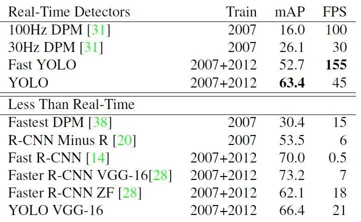
1. PASCAL VOC 2007: Using ZF-Net to train RPN and Fast-R-CNN, the accuracy rates for SelectiveSearch+Fast-R-CNN, EdgeBox+Fast-R-CNN, and RPN+Fast-R-CNN are 58.7%, 58.6%, and 59.9%, respectively. The Selective Search and Edge Box methods extract 2000 proposals, while RPN extracts a maximum of 300 proposals, thus the RPN, which shares convolutional features, clearly has an advantage in efficiency.
2. Training RPN+Fast-R-CNN using VGG with and without shared features yields accuracy rates of 68.5% and 69.9%, respectively (VOC2007). Additionally, when training R-CNN using VGG, it takes 320ms to extract 2000 proposals; with SVD optimization, it takes 223ms; while the entire forward process of Faster-RCNN (including RPN+Fast-R-CNN) only takes 198ms.
3. Although the number of scales and aspect ratios of anchors does not significantly impact results, it is recommended to set both parameters to appropriate values for algorithm stability.
4. When the number of proposals extracted by Selective Search and Edge Box is reduced from 2000 to 300, the recall value in the Recall vs. IoU overlap ratio graph for Fast-R-CNN significantly drops; however, when the number of proposals extracted by RPN is reduced from 2000 to 300, the recall value remains relatively stable.
4.4 Summary
Training RPN+Fast-R-CNN using the shared feature approach achieves excellent detection results, as the shared training of features allows RPN to extract proposals without time cost while enhancing proposal quality. Thus, the alternating training method of RPN+Fast-R-CNN in Faster-R-CNN surpasses the previous Selective Search+Fast-R-CNN.
5. YOLO: You Only Look Once: Unified, Real-Time Object Detection
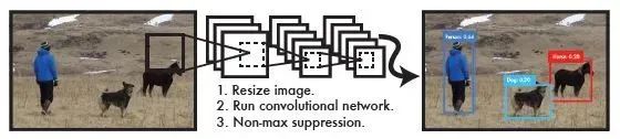
YOLO is a convolutional neural network that can predict multiple box locations and categories in one go, achieving end-to-end object detection and recognition, with its primary advantage being speed. In fact, the essence of object detection is regression, so a CNN that implements regression does not require a complex design process. YOLO does not use sliding windows or proposal extraction methods to train the network; instead, it directly trains the model on the entire image. The benefit of this approach is that it can better distinguish between target and background areas. In contrast, the Fast-R-CNN method that uses proposal training often misidentifies background areas as specific targets. Of course, YOLO sacrifices some accuracy to improve detection speed. The following diagram illustrates the YOLO detection system process: 1. Resize the image to 448*448; 2. Run CNN; 3. Apply non-maximum suppression to optimize detection results. Interested readers can follow the instructions at http://pjreddie.com/darknet/install/ to install and test the YOLO scoring process, which is very easy to get started with. Next, the principles of YOLO will be introduced.
5.1 Integrated Detection Solution
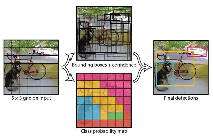
YOLO’s design philosophy adheres to end-to-end training and real-time detection. YOLO divides the input image into S*S networks, where if the center of an object falls within a grid (cell), that grid is responsible for detecting the object. During training and testing, each network predicts B bounding boxes, each corresponding to five predicted parameters: the center coordinates (x,y) of the bounding box, width and height (w,h), and confidence score. The confidence score reflects the likelihood of an object being present in the bounding box (Pr(Object)*IOU(pred|truth)), combining the probability of an object being present and the accuracy of the predicted target location (IOU(pred|truth)). If no object is present within the bounding box, Pr(Object)=0. If an object is present, the IoU is calculated based on the predicted bounding box and the actual bounding box, while the posterior probability of the object belonging to a certain class is predicted as Pr(Class_i|Object). Assuming there are a total of C object classes, each grid only predicts the conditional class probability Pr(Class_i|Object), i=1,2,…,C; each grid predicts B bounding boxes. That is, these B bounding boxes share a set of conditional probabilities Pr(Class_i|Object), i=1,2,…,C. If the input image is divided into 7*7 grids (S=7), and each grid predicts 2 bounding boxes (B=2), with 20 classes of objects to be detected (C=20), it essentially predicts a vector of length S*S*(B*5+C)=7*7*30, thus completing the detection and recognition task. The entire process can be understood through the following diagram.
5.1.1 Network Design
YOLO’s network design follows the principles of GoogleNet but differs in certain aspects. YOLO uses 24 cascaded convolution (conv) layers and 2 fully connected (fc) layers, where the conv layers include 3*3 and 1*1 kernels. The last fc layer is the output of the YOLO network, with a length of S*S*(B*5+C)=7*7*30. In addition, the author also designed a simplified version of the YOLO-small network, which includes 9 cascaded conv layers and 2 fc layers. Due to the significantly fewer conv layers, YOLO-small is much faster than YOLO. The architecture of the YOLO network is illustrated in the following diagram.

5.1.2 Training
The author trains the YOLO network in a stepwise manner: first, they extract the first 20 conv layers from the above network, then add an average pooling layer and a fully connected layer, using the 1000-class ImageNet data for training. After training on ImageNet2012 with images of size 224*224, the top-5 accuracy achieved is 88%. Next, the author adds 4 new conv layers and 2 fc layers after the 20 pre-trained conv layers, initializing the new layers with random parameters. When fine-tuning the new layers, the author uses images of size 448*448 for training. The last fc layer can predict the probabilities of the object belonging to different classes and the center coordinates (x,y) and width and height (w,h) of the bounding box. The width and height of the bounding box are normalized relative to the width and height of the image, while the center coordinates of the bounding box are normalized relative to the position coordinates of a specific grid, thus x,y,w,h are all between 0 and 1.
In designing the loss function, two main issues arise: 1. For the last layer’s predicted results of length 7*7*30, the prediction loss is typically calculated using squared error. However, this loss function has a 1:1 relationship between location error and classification error. 2. The entire image has 7*7 grids, most of which do not contain objects (an object is considered contained only when its center falls within a grid). If only calculating Pr(Class_i), many grids will have a classification probability of 0, resulting in a sparse matrix characteristic for grid loss, which deteriorates the convergence effect and model stability. To address these issues, the author employs a series of solutions:
1. Increase the weight of the bounding box coordinate prediction loss and reduce the weight of the bounding box classification loss. The weights for coordinate prediction and classification prediction are set to λcoord=5, λnoobj=0.5.
2. The squared error for large and small bounding boxes has the same weight; the author uses a square root form to calculate width and height prediction loss, i.e., sqrt(w) and sqrt(h).
The composition of the training loss is quite complex, and will not be listed here; interested readers can refer to the original paper for a slow understanding.
5.1.3 Testing
The author tests the YOLO network trained on PASCAL VOC images, predicting 98 bounding boxes (7*7*2) and corresponding class probabilities for each image. Typically, a cell can directly predict a bounding box corresponding to an object, but for larger objects or those near the image boundary, multiple grid predictions may be needed, which are processed through non-maximum suppression. Although YOLO does not rely on non-maximum suppression as heavily as R-CNN and DPM, it can indeed increase mAP by 2 to 3 points.
5.2 Method Comparison
The author compares the YOLO object detection and recognition method with several classic schemes:
DPM (Deformable Parts Models): DPM is an object detection method based on sliding windows, with a basic process including several independent steps: feature extraction, region division, and predicting bounding boxes based on high-scoring regions. YOLO adopts an end-to-end training approach, connecting feature extraction, candidate box prediction, non-maximum suppression, and object recognition into a faster and more accurate detection model.
R-CNN: The R-CNN scheme first requires using the Selective Search method to extract proposals, then uses CNN for feature extraction, and finally trains the classifier using SVM. This scheme is quite cumbersome! The essence of YOLO is similar, but it extracts proposals and recognizes targets by sharing convolutional features. Additionally, YOLO constrains proposals spatially using grids, avoiding repeated proposal extraction in certain areas. Compared to R-CNN, which extracts 2000 proposals for training, YOLO only needs to extract 98 proposals, making training and testing much faster.
Fast-R-CNN, Faster-R-CNN, Fast-DPM: Fast-R-CNN and Faster-R-CNN replaced the SVM training and Selective Search proposal extraction methods, respectively, speeding up training and testing to some extent, but their speed still cannot compare to YOLO. Similarly, optimizing DPM for GPU implementation does not surpass YOLO.
5.3 Experiments
5.3.1 Comparison of Real-Time Detection and Recognition Systems
5.3.2 VOC2007 Accuracy Comparison
5.3.3 Error Analysis of Fast-R-CNN and YOLO
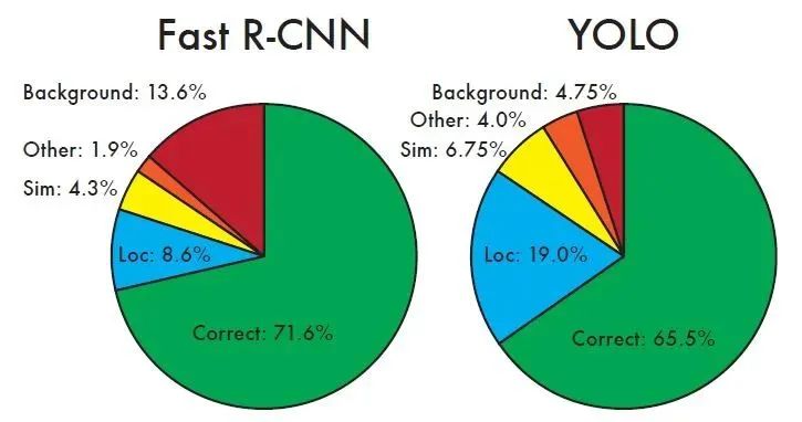
As shown in the figure, different areas represent different metrics:
Correct: The proportion of correctly detected and recognized instances, i.e., correct classification with IOU>0.5
Localization: Correct classification, but 0.1<IOU<0.5
Similar: Similar categories, IOU>0.1
Other: Incorrect classification, IOU>0.1
Background: For any target, IOU<0.1
It can be seen that YOLO’s accuracy in locating target positions is not as high as that of Fast-R-CNN. The proportion of target localization errors in YOLO’s errors is the highest, exceeding Fast-R-CNN by 10 points. However, YOLO has a higher accuracy in recognizing backgrounds, indicating that Fast-R-CNN has a high false positive rate (Background=13.6%, meaning it identifies a box as a target, but it actually contains no object).
5.3.4 VOC2012 Accuracy Comparison
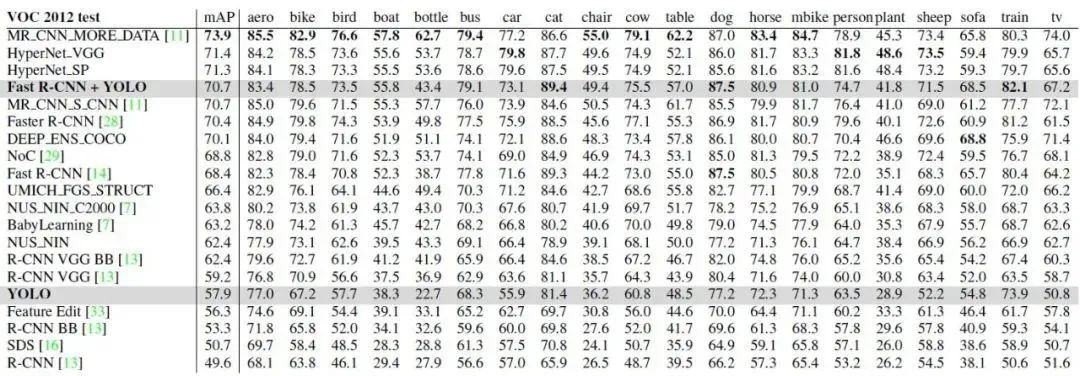
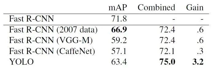
Since YOLO shows more advantages in recognizing background parts during object detection and recognition, the author designed a Fast-R-CNN+YOLO detection and recognition mode, which first uses R-CNN to extract a set of bounding boxes, then uses YOLO to process the image to obtain another set of bounding boxes. Comparing these two sets of bounding boxes for consistency, if they match, the probability calculated by YOLO is used for target classification, and the final bounding box is selected from the intersection area of both. The highest accuracy of Fast-R-CNN can reach 71.8%, while using Fast-R-CNN+YOLO can improve the accuracy to 75.0%. This improvement in accuracy is based on the fact that YOLO makes different errors at the testing end compared to Fast-R-CNN. Although Fast-R-CNN_YOLO improves accuracy, the corresponding detection and recognition speed decreases significantly, making it impossible for real-time detection.
Using VOC2012 to test the mean Average Precision of different algorithms, YOLO’s mAP=57.9%, which is comparable to the accuracy rate of the R-CNN detection algorithm based on VGG16. Regarding the testing effects of images of different sizes, the author found that YOLO’s accuracy in detecting small targets is about 8-10% lower than that of R-CNN, while its accuracy in detecting large targets is higher than that of R-CNN. The method of Fast-R-CNN+YOLO achieves the highest accuracy, exceeding that of Fast-R-CNN by 2.3%.
5.4 Summary
YOLO is a convolutional neural network that supports end-to-end training and testing, enabling detection and recognition of multiple targets in images while maintaining a certain level of accuracy.
Download 1: OpenCV-Contrib Extension Module Chinese Version Tutorial

Reply "Extension Module Chinese Tutorial" in the "Beginner's Guide to Vision" public account backend to download the first Chinese version of the OpenCV extension module tutorial online, covering installation of extension modules, SFM algorithms, stereo vision, target tracking, biological vision, super-resolution processing, etc. over twenty chapters of content.

Download 2: Python Vision Practical Project 52 Lectures

Reply "Python Vision Practical Project" in the "Beginner's Guide to Vision" public account backend to download 31 practical vision projects, including image segmentation, mask detection, lane line detection, vehicle counting, eyeliner addition, license plate recognition, character recognition, emotion detection, text content extraction, facial recognition, etc., to assist in quickly learning computer vision.

Download 3: OpenCV Practical Project 20 Lectures

Reply "OpenCV Practical Project 20 Lectures" in the "Beginner's Guide to Vision" public account backend to download 20 practical projects based on OpenCV, advancing OpenCV learning.

Discussion Group

Welcome to join the public account reader group to communicate with peers; there are currently WeChat groups for SLAM, 3D vision, sensors, autonomous driving, computational photography, detection, segmentation, recognition, medical imaging, GAN, algorithm competitions, etc. (will gradually be subdivided in the future). Please scan the WeChat ID below to join the group, with the note: "Nickname + School/Company + Research Direction", for example: "Zhang San + Shanghai Jiao Tong University + Visual SLAM". Please follow the format; otherwise, you will not be allowed to join. After successful addition, you will be invited to the relevant WeChat group based on your research direction. Please do not send advertisements in the group; otherwise, you will be removed from the group. Thank you for your understanding~