A Small Change: CNN Input from Fixed to Variable Image Sizes

Click on the aboveBeginner Learning Vision“, select to add “Star” or “Top

Essential content delivered promptlyA Small Change: CNN Input from Fixed to Variable Image Sizes

In this article, we will learn how to classify images of any size without using computationally intensive sliding windows. By modifying the ResNet-18 CNN framework, we will change the required input size from 224×224 to any size.
First, we clarify a common misconception about Convolutional Neural Networks (CNNs).
Convolutional Neural Networks do not require fixed-size inputs
If we have used CNNs for image classification, we need to crop or resize the input image to meet the required input size of the CNN network. Although this practice is very common, there are some limitations to using this method.
1. Resolution Decrease: If there is a small dog in a large image but it only occupies a small part of the image, resizing the image will make the dog smaller to the point where it cannot be correctly classified.
2. Non-Square Aspect Ratio: Typically, image classification networks are trained on square images. If the input image is not square, we generally take a square region from the center or use different ratios to adjust the width and height to make the image square. In the first case, we may ignore important features that are not centered. In the second case, image information may be distorted due to uneven scaling.
3. High Computational Load: To solve this problem, we can overlap crop the image and perform image classification on each window. This is computationally intensive and completely unnecessary.
Interestingly, many people do not realize that if we make small modifications to the network, CNNs can accept images of any size as input without needing to retrain! In this article, we will introduce how to achieve input of images of any size by modifying a standard network example.
Modifying the Image Classification Architecture to Handle Arbitrary Size Images
Almost all classification architectures have a fully connected layer (FC) at the end. (Note: The FC layer is referred to as a “linear” layer in PyTorch.) The problem with FC layers is that they require fixed-size input data. If we change the size of the input image, calculations cannot be performed. Therefore, we need to replace the FC layer with something else, but before that, we need to understand why fully connected layers are needed in image classification architectures.
Modern CNN architectures consist of several convolutional layer blocks followed by a few FC layers. This structure can be traced back to the early research of neural networks. Convolutional layers act as “smart” filters to extract semantic information from images, retaining spatial relationships between objects in the image to some extent. However, to classify objects in an image, we do not need this spatial information, so the output of the last convolutional layer is usually flattened into a long vector. This long vector serves as the input to the FC layer, which does not consider spatial information. FC layers only perform weighted summation of deep features across all spatial locations in the image.
In practice, this structure performs well and has been validated through extensive practice. However, due to the presence of FC layers, the network can only accept fixed-size inputs. Therefore, we need to replace the FC layer with a type of network layer that does not require fixed-size inputs. This is the convolutional layer that is not limited by its input size!
Next, we will use an equivalent convolutional layer to replace the FC layer.
Converting Fully Connected Layers to Convolutional Layers
FC and convolutional layers differ in their target inputs – convolutional layers focus on local input regions, while FC layers combine global features. However, both FC and convolutional layers calculate dot products, so they are inherently similar. Thus, the conditions for mutual conversion between the two are satisfied.
We will explain this with an example.
Assume there is an FC layer that takes the output of a convolutional layer as input, and the convolutional layer outputs a tensor of size 5x5x16. We also assume that the output size of the FC layer is 120. If using an FC layer, we first flatten the volume of 5x5x16 into a vector of size 400×1 (i.e., 5x5x16). However, using the equivalent convolutional layer, we need to use a kernel of size 5x5x16. In CNNs, the depth of the kernel (in this case, 16) is always the same as the depth of the input, and the width and height are generally the same (in this case, 5). Therefore, we can simply say the kernel size is 5, rather than 5x5x16. The number of filters needs to match the desired output, so it is set to 120. At the same time, the stride is set to 1, and padding to 0.
Modifying the ResNet-18 Architecture
ResNet-18 is a popular CNN architecture that requires input images of size 224×224. However, we will modify it to accept inputs of arbitrary sizes.
The following diagram shows the composition of the framework
A Small Change: CNN Input from Fixed to Variable Image Sizes
In PyTorch, the ResNet-18 architecture starts with a convolutional layer called conv1 (see the code below). Then comes the pooling layer.
Next, there are 4 convolutional blocks, which are shown in pink, purple, yellow, and orange in the figure. These modules are named layer1, layer2, layer3, and layer4. Each module contains 4 convolutional layers.
Finally, we have an average pooling layer. The output of this layer is flattened and sent to the final fully connected layer FC.
The following code is the implementation of the ResNet framework.
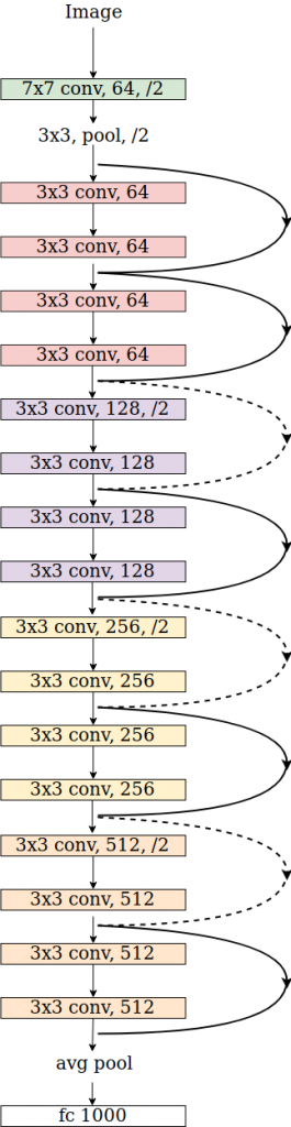
# from the torchvision's implementation of ResNet
class ResNet:
   # ...   self.conv1 = nn.Conv2d(3, self.inplanes, kernel_size=7, stride=2, padding=3,                              bias=False)       self.bn1 = norm_layer(self.inplanes)       self.relu = nn.ReLU(inplace=True)       self.maxpool = nn.MaxPool2d(kernel_size=3, stride=2, padding=1)       self.layer1 = self._make_layer(block, 64, layers[0])       self.layer2 = self._make_layer(block, 128, layers[1], stride=2, dilate = replace_stride_with_dilation[0])       self.layer3 = self._make_layer(block, 256, layers[2], stride=2, dilate = replace_stride_with_dilation[1])       self.layer4 = self._make_layer(block, 512, layers[3], stride=2, dilate = replace_stride_with_dilation[2])       self.avgpool = nn.AdaptiveAvgPool2d((1, 1))       self.fc = nn.Linear(512 * block.expansion, num_classes)
   # ...
   def _forward_impl(self, x):       # See note [TorchScript super()]
       x = self.conv1(x)       x = self.bn1(x)       x = self.relu(x)       x = self.maxpool(x)
       x = self.layer1(x)       x = self.layer2(x)       x = self.layer3(x)       x = self.layer4(x)
       x = self.avgpool(x)       x = torch.flatten(x, 1)       x = self.fc(x)
       return x
We will create a new class FullyConvolutionalResnet18 by inheriting from the original ResNet class, with the following code:
class FullyConvolutionalResnet18(models.ResNet):   def __init__(self, num_classes=1000, pretrained=False, **kwargs):
       # Start with standard resnet18 defined here       super().__init__(block = models.resnet.BasicBlock, layers = [2, 2, 2, 2], num_classes = num_classes, **kwargs)       if pretrained:           state_dict = load_state_dict_from_url( models.resnet.model_urls["resnet18"], progress=True)           self.load_state_dict(state_dict)
       # Replace AdaptiveAvgPool2d with standard AvgPool2d       self.avgpool = nn.AvgPool2d((7, 7))
       # Convert the original fc layer to a convolutional layer.         self.last_conv = torch.nn.Conv2d( in_channels = self.fc.in_features, out_channels = num_classes, kernel_size = 1)       self.last_conv.weight.data.copy_( self.fc.weight.data.view ( *self.fc.weight.data.shape, 1, 1))       self.last_conv.bias.data.copy_ (self.fc.bias.data)
   # Reimplementing forward pass.   def _forward_impl(self, x):       # Standard forward for resnet18       x = self.conv1(x)       x = self.bn1(x)       x = self.relu(x)       x = self.maxpool(x)
       x = self.layer1(x)       x = self.layer2(x)       x = self.layer3(x)       x = self.layer4(x)       x = self.avgpool(x)
       # Notice, there is no forward pass       # through the original fully connected layer.       # Instead, we forward pass through the last conv layer       x = self.last_conv(x)       return x
Using Fully Convolutional ResNet-18
With our definition, we now have a ResNet-18 capable of processing images of any size. Next, we will introduce how to use our newly defined ResNet-18.
#1. Import standard libraries
import torch
import torch.nn as nn
from torchvision import models
from torch.hub import load_state_dict_from_url
from PIL import Image
import cv2
import numpy as np
from matplotlib import pyplot as plt

#2. Read ImageNet class ID to name mapping
if __name__ == "__main__":
   # Read ImageNet class id to name mapping   with open('imagenet_classes.txt') as f:       labels = [line.strip() for line in f.readlines()]
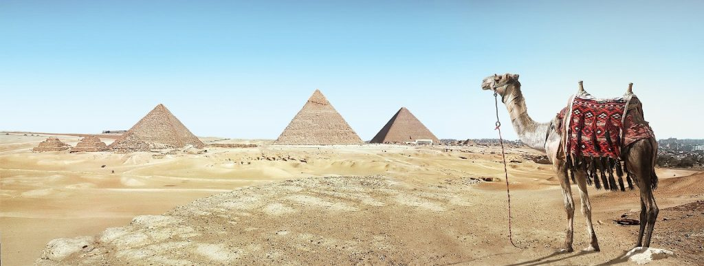
Read the image and convert it to a format that can be used with PyTorch.
A Small Change: CNN Input from Fixed to Variable Image Sizes
Input image: Note that the camel is not centered in the image
# Read image
original_image = cv2.imread('camel.jpg')
# Convert original image to RGB format
image = cv2.cvtColor(original_image, cv2.COLOR_BGR2RGB)
# Transform input image
# 1. Convert to Tensor
# 2. Subtract mean
# 3. Divide by standard deviation
transform = transforms.Compose([                        transforms.ToTensor(), #Convert image to tensor.            transforms.Normalize(                                  mean=[0.485, 0.456, 0.406],   # Subtract mean            std=[0.229, 0.224, 0.225]     # Divide by standard deviation                        )])
image = transform(image)
image = image.unsqueeze(0)
Load the Fully Convolutional ResNet-18 model with pretrained parameters.
# Load modified resnet18 model with pretrained ImageNet weights
model = FullyConvolutionalResnet18(pretrained=True).eval()
Perform network computation to obtain results
with torch.no_grad():   # Perform inference.   # Instead of a 1x1000 vector, we will get a   # 1x1000xnxm output ( i.e. a probability map   # of size n x m for each 1000 class,   # where n and m depend on the size of the image.)   preds = model(image)   preds = torch.softmax(preds, dim=1)
   print('Response map shape : ', preds.shape)
   # Find the class with the maximum score in the n x m output map   pred, class_idx = torch.max(preds, dim=1)   print(class_idx)
   row_max, row_idx = torch.max(pred, dim=1)   col_max, col_idx = torch.max(row_max, dim=1)   predicted_class = class_idx[0, row_idx[0, col_idx], col_idx]
   # Print top predicted class   print('Predicted Class : ', labels[predicted_class], predicted_class)
When we run the above code, we will get the following output.
Response map shape :  torch.Size([1, 1000, 3, 8])
tensor([[[977, 977, 977, 977, 977, 978, 354, 437],        [978, 977, 980, 977, 858, 970, 354, 461],        [977, 978, 977, 977, 977, 977, 354, 354]]])
Predicted Class :  Arabian camel, dromedary, Camelus dromedarius tensor([354])
In the original ResNet, the output is a vector of 1000 elements, where each element corresponds to the class probabilities of 1000 classes in ImageNet.
In the FC version, we get a response map of size [1, 1000, n, m], where n and m depend on the original size of the image and the network itself.
In our example, when we input an image of size 1920×725, we receive a response map of size [1, 1000, 3, 8].
Response map for predicted class
Next, we find the response map for the predicted class and upsample it to fit the original image. We threshold the response map to obtain the region of interest and find a bounding box around it. The specific code is as follows:
# Find the n x m score map for the predicted class
score_map = preds[0, predicted_class, :, :].cpu().numpy()
score_map = score_map[0]
# Resize score map to the original image size
score_map = cv2.resize(score_map, (original_image.shape[1], original_image.shape[0]))
# Binarize score map_, score_map_for_contours = cv2.threshold(score_map, 0.25, 1, type=cv2.THRESH_BINARY)
score_map_for_contours = score_map_for_contours.astype(np.uint8).copy()
# Find the contour of the binary blob
contours, _ = cv2.findContours(score_map_for_contours, mode=cv2.RETR_EXTERNAL, method=cv2.CHAIN_APPROX_SIMPLE)
# Find bounding box around the object.
rect = cv2.boundingRect(contours[0])
Display results
The following code is used to display results in image form. The brighter areas in the response map indicate high probability regions.
# Apply score map as a mask to original image
score_map = score_map - np.min(score_map[:])
score_map = score_map / np.max(score_map[:])
Next, we will multiply the response map with the original image and display the bounding box.
score_map = cv2.cvtColor(score_map, cv2.COLOR_GRAY2BGR)
masked_image = (original_image * score_map).astype(np.uint8)
# Display bounding box
cv2.rectangle(masked_image, rect[:2], (rect[0] + rect[2], rect[1] + rect[3]), (0, 0, 255), 2)
# Display images
cv2.imshow("Original Image", original_image)
cv2.imshow("scaled_score_map", score_map)
cv2.imshow("activations_and_bbox", masked_image)
cv2.waitKey(0)
The results are shown below. We see that only the camel is highlighted. The bounding box created by thresholding the response map captures the camel. In this sense, the fully convolutional image classifier acts like an object detector!
A Small Change: CNN Input from Fixed to Variable Image Sizes
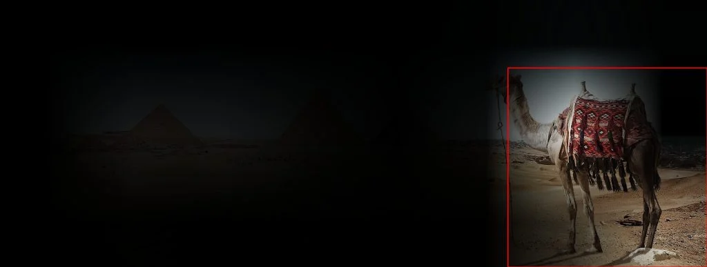
Download 1: OpenCV-Contrib Extension Module Chinese Tutorial
Reply: Extension Module Chinese Tutorial in the "Beginner Learning Vision" public account background to download the first OpenCV extension module tutorial in Chinese, covering more than twenty chapters including extension module installation, SFM algorithms, stereo vision, object tracking, biological vision, super-resolution processing, etc.

Download 2: Python Vision Practical Projects 52 Lectures
Reply: Python Vision Practical Projects in the "Beginner Learning Vision" public account background to download 31 visual practical projects including image segmentation, mask detection, lane line detection, vehicle counting, adding eyeliner, license plate recognition, character recognition, emotion detection, text content extraction, face recognition, etc., to help quickly learn computer vision.

Download 3: OpenCV Practical Projects 20 Lectures
Reply: OpenCV Practical Projects 20 Lectures in the "Beginner Learning Vision" public account background to download 20 practical projects based on OpenCV for advanced learning of OpenCV.

Discussion Group

Welcome to join the public account reader group to communicate with peers. Currently, we have WeChat groups for SLAM, 3D vision, sensors, autonomous driving, computational photography, detection, segmentation, recognition, medical imaging, GAN, algorithm competitions, etc. (will gradually subdivide in the future). Please scan the WeChat ID below to join the group, and note: "Nickname + School/Company + Research Direction", for example: "Zhang San + Shanghai Jiao Tong University + Vision SLAM". Please follow the format for remarks, otherwise, it will not be approved. After successful addition, you will be invited to the relevant WeChat group based on your research direction. Please do not send advertisements in the group, otherwise, you will be removed from the group. Thank you for your understanding~

Leave a Comment