An Overview of Convolutional Neural Networks and Analysis of ImageNet Champion Models

Convolutional Neural Networks (CNN) were originally designed to solve problems such as image recognition. However, their applications are not limited to images and videos; they can also be used for time series signals, such as audio signals and text data. In early image recognition research, the biggest challenge was how to organize features, as image data cannot be easily understood and features extracted manually like other types of data.

In models like stock prediction, we can extract past trading price fluctuations, price-earnings ratios, price-to-book ratios, and earnings growth from raw data; this is called feature engineering. However, in images, it is challenging to extract effective and rich features based on human understanding. Before the advent of deep learning, we had to rely on algorithms such as SIFT and HoG to extract features with good discriminative power, and then combine them with machine learning algorithms like SVM for image recognition.

SIFT is invariant to distortions such as scaling, translation, rotation, perspective changes, and brightness adjustments to a certain extent, making it one of the most important image feature extraction methods at that time. However, algorithms like SIFT still have limitations, with the best error rate in the ImageNet ILSVRC competition being over 26%, and breakthroughs were hard to come by for years.

The features extracted by convolutional neural networks can achieve better results, and they do not require separating the feature extraction and classification training processes; they automatically extract the most effective features during training. The initial goal of proposing CNN as a deep learning architecture was to reduce the requirements for image data preprocessing and to avoid complex feature engineering. CNN can directly use raw pixel data from images as input, without needing to extract features using algorithms like SIFT first, which reduces the amount of repetitive and tedious data preprocessing that traditional algorithms such as SVM require.

Similar to algorithms like SIFT, the models trained by CNN are also invariant to distortions such as scaling, translation, and rotation, exhibiting strong generalization capabilities. The most significant feature of CNN is its weight-sharing structure in convolution, which can greatly reduce the number of parameters in the neural network, preventing overfitting while also reducing the complexity of the neural network model.

The concept of convolutional neural networks originated from the receptive field proposed by scientists in the 1960s. Scientists discovered through studies of the visual cortex cells of cats that each visual neuron processes only a small area of the visual image, known as the receptive field. In the 1980s, Japanese scientists introduced the concept of the Neocognitron, which can be considered an early prototype of convolutional networks.

The Neocognitron contains two types of neurons: S-cells for feature extraction and C-cells for deformation resistance. The S-cells correspond to the convolutional operations in our current mainstream CNNs, while the C-cells correspond to activation functions, max pooling, and other operations. Moreover, CNN was the first network structure to successfully perform multi-layer training, as mentioned in the previous chapters regarding LeCun’s LeNet5. In contrast, fully connected networks faced challenges in multi-layer training due to excessive parameters and gradient vanishing issues.

Convolutional neural networks can leverage spatial structural relationships to reduce the number of parameters to be learned, thereby improving the training efficiency of the backpropagation algorithm. In a convolutional neural network, the first convolutional layer directly accepts pixel-level input from images. Each convolution operation processes only a small portion of the image, and after convolution, the results are passed to subsequent networks. Each convolution layer (or filter) extracts the most effective features from the data. This method can capture the most basic features in images, such as edges or corners in various directions, and then combine and abstract them to form higher-order features. Therefore, CNN can handle various situations and theoretically possesses invariance to image scaling, translation, and rotation.

A typical convolutional neural network consists of multiple convolutional layers, with each layer usually performing the following operations:

1. The image is filtered through multiple different convolutional kernels and biases to extract local features, with each convolutional kernel mapping to a new 2D image.

2. The output from the previous convolutional kernel filtering is processed using a nonlinear activation function. Currently, the most common is the ReLU function, while the Sigmoid function was more widely used in the past.

3. The results of the activation function are further processed through pooling operations (i.e., downsampling, such as reducing a 2×2 image to a 1×1 image), typically using max pooling to retain the most significant features and enhance the model’s tolerance to distortions.

A convolutional layer can have multiple different convolutional kernels, and each kernel corresponds to a new image mapped after filtering. Each pixel in the same new image comes from the same convolutional kernel, which is the concept of weight sharing of convolutional kernels. So why do we share the weight parameters of convolutional kernels? The answer is simple: to reduce model complexity, mitigate overfitting, and decrease computational load.

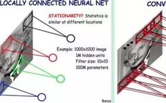
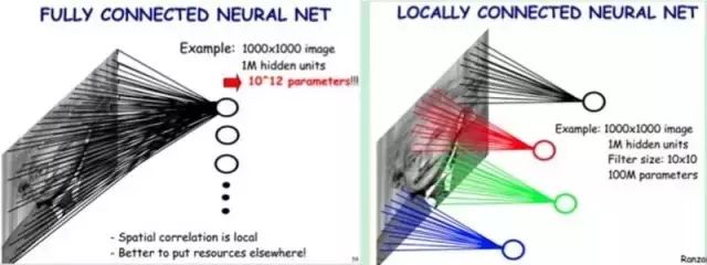
For example, as shown in Figure 5-2, if our image size is 1000 pixels × 1000 pixels and we assume it is a grayscale image (i.e., only one color channel), then a single image has 1 million pixels, and the input data dimension is also 1 million. Next, if we connect a hidden layer of the same size (1 million hidden nodes), it will produce 1 million × 1 million = 1 trillion connections.

Just one fully connected layer has 1 trillion connection weights to train, which exceeds the computational capability of ordinary hardware. We must reduce the number of weights to be trained for two reasons: to reduce computational complexity and to mitigate severe overfitting, as excessive connections can impair the model’s generalization ability.

Images are organized spatially, and each pixel is closely related to nearby pixels, but may not have any correlation with distant pixels. This relates to the previously mentioned concept of the human visual receptive field, where each receptive field only receives signals from a small area. The pixels within this small area are interrelated, and each neuron does not need to receive information from all pixel points, but only needs to receive local pixel information as input. The cumulative information from these local neurons can yield global information.

This allows us to modify the previous fully connected model to a local connection model. Previously, each hidden node was connected to all pixels, but now we only need to connect each hidden node to local pixel nodes. Assuming the local receptive field size is 10×10, meaning each hidden node connects to 10×10 pixel points, we now only need 10×10 × 1 million = 100 million connections, a reduction of 10,000 times from the previous 1 trillion.

In simple terms, the left part of the figure represents fully connected, while the right part represents local connections. Local connections can drastically reduce the number of parameters in the neural network, from 100M × 100M = 1 trillion to 10 × 10 × 1 million = 100 million.

In the previous example, we used local connections to reduce the number of connections from 1 trillion to 100 million, but it is still too many, and we need to continue reducing the number of parameters. Now, each node in the hidden layer connects to 10 × 10 pixels, meaning each hidden node has 100 parameters. If our local connection method is convolution, meaning each hidden node’s parameters are identical, our parameters are no longer 100 million but just 100. Regardless of how large the image is, the number of parameters is only related to the size of the convolutional kernel, which is the contribution of convolution to reducing the parameter count.

In simple terms, convolution uses the same (identical parameters) template for local connections, allowing the parameter count to drop dramatically.

We no longer need to worry about how many hidden nodes there are or how large the image is; the number of parameters only relates to the size of the convolutional kernel, which is known as weight sharing. However, if we only have one convolutional kernel, we can only extract one type of convolutional filtering result, meaning we can only extract one type of image feature, which is not our desired outcome. Fortunately, the most basic features in images are few, and we can increase the number of convolutional kernels to extract more features.

The basic features in images are merely points and edges; no matter how complex an image is, it is composed of combinations of points and edges. The way the human eye recognizes objects also starts with points and edges. Visual neurons receive light signals, with each neuron receiving signals from only a localized area, extracting features of points and edges, and then passing the signals of points and edges to the next layer of neurons, which further combine them into higher-order features, such as triangles, squares, lines, and corners, eventually abstracting and combining them into facial features like eyes, nose, and mouth, culminating in recognizing a face.

Thus, our problem is easily solved; as long as we provide enough convolutional kernels, capable of extracting edges in various directions or points of various shapes, we can allow the convolutional layer to abstract effective and rich higher-order features. The image obtained from the filtering of each convolutional kernel is a mapping of a feature type, known as a Feature Map. Generally, using 100 convolutional kernels in the first convolutional layer is already sufficient.

In this case, as shown in the figure above, our parameter count is 100 × 100 = 10,000, a reduction of 10,000 times from the previous 100 million. Therefore, thanks to convolution, we can efficiently train a neural network with local connections. The benefit of convolution is that regardless of the image size, the number of weights we need to train only relates to the size and number of convolutional kernels, allowing us to process images of any size with a very small number of parameters. Each convolutional layer extracts features that are abstracted and combined into higher-order features in subsequent layers.

To summarize, the key points of convolutional neural networks are local connection, weight sharing, and down-sampling in pooling layers.

Local connections and weight sharing reduce the parameter count, significantly decreasing training complexity and alleviating overfitting. At the same time, weight sharing grants convolutional networks tolerance to translation, while pooling layers’ down-sampling further reduces the output parameter count and provides the model with tolerance to slight deformations, enhancing the model’s generalization capability.

Compared to traditional machine learning algorithms, CNNs do not require manual feature extraction and do not need to use feature extraction algorithms like SIFT; they can automatically complete feature extraction and abstraction during training while simultaneously performing pattern classification, greatly reducing the difficulty of applying image recognition. Compared to general neural networks, CNNs are structurally closer to the spatial structure of images, both being 2D connected structures, and the convolutional connection method of CNN is similar to how human visual neurons process light signals.

The following introduces the classic convolutional network LeNet5.

The renowned LeNet5 was born in 1994 and is one of the earliest deep convolutional neural networks, significantly advancing deep learning. Starting from 1988, after several successful iterations, this pioneering achievement completed by Yann LeCun was named LeNet5.

LeCun believed that trainable parameter convolutional layers are an effective way to extract similar features at multiple positions in images with a small number of parameters, which is different from directly using each pixel as input for a multilayer neural network. Pixels should not be used in the input layer because images have strong spatial correlations, and using independent pixels directly as input fails to utilize these correlations.

The characteristics of LeNet5 at that time included:

• Each convolutional layer consists of three parts: convolution, pooling, and nonlinear activation functions.

• Uses convolution to extract spatial features.

• Subsample using average pooling.

• Uses hyperbolic tangent (Tanh) or sigmoid activation functions.

• MLP as the final classifier.

• Sparse connections between layers reduce computational complexity.

Many features of LeNet5 are still used in state-of-the-art convolutional neural networks today, making it a foundational work for modern convolutional neural networks. The structure of LeNet-5 is shown in the figure below:

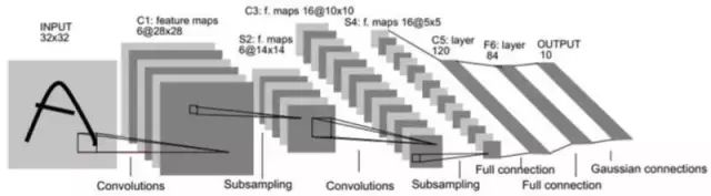
Its input image is a 32×32 grayscale image, followed by 3 convolutional layers, 1 fully connected layer, and 1 Gaussian connected layer.

Next, we will introduce some other classic convolutional network architectures: AlexNet, VGGNet, Google Inception Net, and ResNet. These four networks are arranged in the order of their emergence, with increasing depth and complexity.

They won the classification project of the ILSVRC (ImageNet Large Scale Visual Recognition Challenge) in 2012 (AlexNet, top-5 error rate 16.4%, can reach 15.3% using additional data, 8-layer neural network), 2014 runner-up (VGGNet, top-5 error rate 7.3%, 19-layer neural network), 2014 champion (InceptionNet, top-5 error rate 6.7%, 22-layer neural network), and 2015 champion (ResNet, top-5 error rate 3.57%, 152-layer neural network).

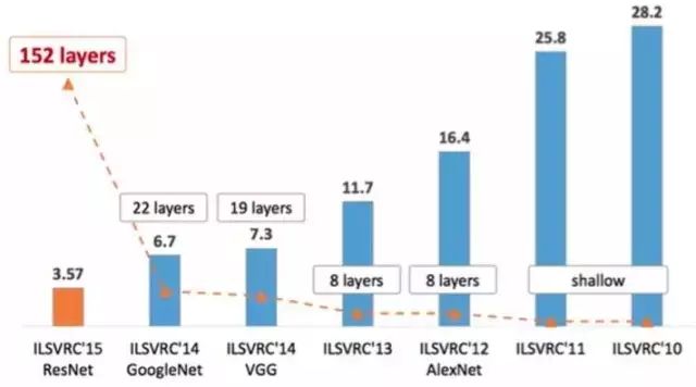
As shown in the figure, the top-5 error rates of ILSVRC have made significant breakthroughs in recent years, with the major breakthroughs being in deep learning and convolutional neural networks, where significant improvements in performance have almost always been accompanied by an increase in the depth of convolutional neural networks.

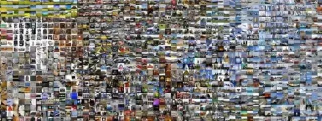
The data used in the computer vision competition ILSVRC comes from ImageNet, as shown in the figure. The ImageNet project was founded in 2007 by Stanford University professor Fei-Fei Li, aiming to collect a large number of labeled images for training computer vision models. ImageNet has 15 million labeled high-definition images, totaling 22,000 categories, with about 1 million images labeled with bounding boxes for the main objects in the images.

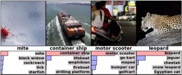
Each year’s ILSVRC competition dataset contains approximately 1.2 million images and 1,000 labeled categories, which is a subset of all ImageNet data. The competition generally uses top-5 and top-1 classification error rates as performance evaluation metrics for models. The figure shows how AlexNet recognized images in the ILSVRC dataset, with the top five predicted categories and their scores displayed below each image.

AlexNet is the foundation of modern deep CNNs.

In 2012, Hinton’s student Alex Krizhevsky proposed the deep convolutional neural network model AlexNet, which can be considered a deeper and wider version of LeNet. AlexNet included several new technical points and successfully applied ReLU, Dropout, and LRN tricks in CNN for the first time. AlexNet also utilized GPUs for computation acceleration, and the authors open-sourced their CUDA code for training convolutional neural networks on GPUs.

AlexNet contains 630 million connections, 60 million parameters, and 650,000 neurons, with 5 convolutional layers, 3 of which are followed by max pooling layers, and finally 3 fully connected layers. AlexNet won the fiercely competitive ILSVRC 2012 competition with a significant advantage, reducing the top-5 error rate to 16.4%, a huge improvement over the 26.2% error rate of the second place.

AlexNet can be seen as the first voice of neural networks after a low period, establishing the dominance of deep learning (deep convolutional networks) in computer vision, and also promoting the expansion of deep learning into fields such as speech recognition, natural language processing, and reinforcement learning.

AlexNet expanded upon the ideas of LeNet, applying the basic principles of CNN to a very deep and wide network. The main new technical points used in AlexNet are as follows:

1. Successfully used ReLU as the activation function for CNN, demonstrating that its effectiveness surpasses that of Sigmoid in deeper networks, effectively solving the vanishing gradient problem associated with Sigmoid in deeper networks. Although the ReLU activation function was proposed long before, it was not until the advent of AlexNet that it gained prominence.

2. During training, Dropout randomly ignores a portion of neurons to avoid model overfitting. While Dropout has been discussed in a separate paper, AlexNet operationalized it and confirmed its effectiveness through practice. In AlexNet, Dropout was mainly used in the last few fully connected layers.

3. Used overlapping max pooling in CNN. Previously, average pooling was commonly used in CNN; AlexNet exclusively used max pooling to avoid the blurring effect of average pooling. Moreover, AlexNet proposed that the stride should be smaller than the pooling kernel size, resulting in overlapping and coverage between the outputs of the pooling layers, enhancing the richness of features.

4. Introduced LRN layers to create a competitive mechanism for the activity of local neurons, making larger responses relatively larger while suppressing smaller feedback from other neurons, thus enhancing the model’s generalization ability.

5. Utilized CUDA to accelerate the training of deep convolutional networks, leveraging the powerful parallel computing capabilities of GPUs to handle the extensive matrix operations required during neural network training. AlexNet used two GTX 580 GPUs for training, with each GTX 580 having only 3GB of memory, limiting the maximum scale of the trainable network. Therefore, the authors distributed AlexNet across two GPUs, storing half of the parameters of the neurons in the memory of each GPU.

6. Data augmentation, randomly cropping 224×224 regions from the original 256×256 images (and flipping them horizontally), effectively increasing the data volume by (256-224)^2 * 2 = 2048 times. Without data augmentation, the CNN with numerous parameters would fall into overfitting; using data augmentation significantly alleviates overfitting and enhances generalization ability. During prediction, the four corners and the center of the image are taken, totaling 5 positions, with left-right flips, resulting in 10 images for prediction and averaging the results of the 10 predictions.

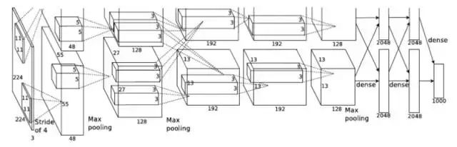
The entire AlexNet has 8 layers requiring training parameters (excluding pooling and LRN layers), with the first 5 layers being convolutional layers and the last 3 layers being fully connected layers, as shown in the figure. The last layer of AlexNet is a Softmax layer with 1000 outputs for classification. LRN layers appear after the first and second convolutional layers, while max pooling layers appear after the two LRN layers and the last convolutional layer.

The hyperparameters, parameter counts, and computational loads of each layer in AlexNet are illustrated in the figure. We can observe an interesting phenomenon: in the early convolutional layers, while the computational load is high, the parameter count is low, all around 1 million or even less, accounting for a small portion of AlexNet’s total parameter count. This is the utility of convolutional layers, which can extract effective features with a small number of parameters.

Although each convolutional layer accounts for less than 1% of the total parameter count of the network, removing any convolutional layer would significantly decrease the network’s classification performance.

VGGNet was developed by researchers from the Visual Geometry Group at the University of Oxford and Google DeepMind. VGGNet explored the relationship between the depth of convolutional neural networks and their performance by repeatedly stacking small 3×3 convolutional kernels and 2×2 max pooling layers, successfully constructing convolutional neural networks with depths of 16 to 19 layers. Compared to previous state-of-the-art network structures, VGGNet significantly reduced error rates and achieved 2nd place in the classification project and 1st place in the localization project of the ILSVRC 2014 competition.

In the VGGNet paper, all layers used 3×3 convolutional kernels and 2×2 pooling kernels, enhancing performance by deepening the network structure. The figure below illustrates the network structure of VGGNet at each level, along with detailed performance testing from 11-layer to 19-layer networks.

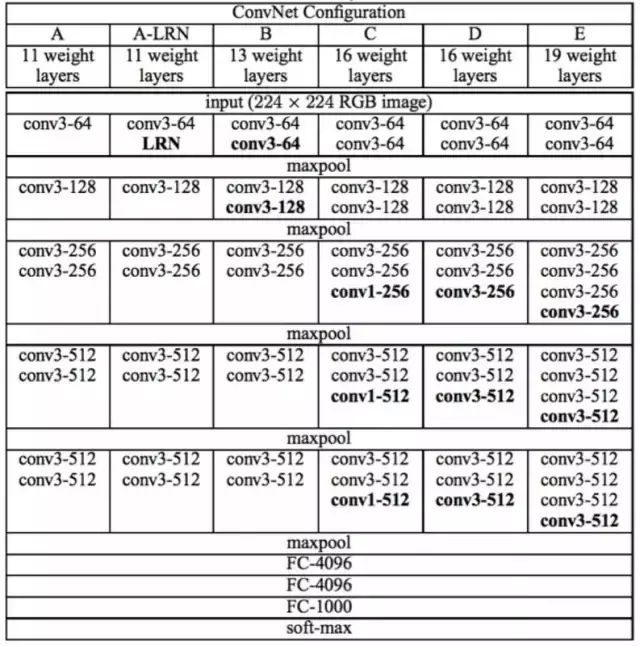
Although the networks from A to E gradually become deeper, the parameter count does not increase significantly, primarily because most parameters are consumed in the last three fully connected layers. The convolutional portions at the front, while deep, do not consume many parameters; however, the training remains time-consuming due to the high computational load of convolutions.

VGGNet consists of 5 segments of convolutions, with 2 to 3 convolutional layers in each segment, and each segment ends with a max pooling layer to reduce the image size. The number of convolutional kernels is the same within each segment, increasing in later segments: 64 – 128 – 256 – 512 – 512. It is common to see multiple identical 3×3 convolutional layers stacked together, which is a very useful design.

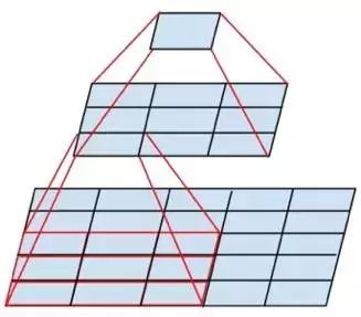
As shown in the figure, two 3×3 convolutional layers in series are equivalent to one 5×5 convolutional layer, meaning a pixel will relate to surrounding 5×5 pixels, effectively increasing the receptive field to 5×5. A series of three 3×3 convolutional layers is equivalent to one 7×7 convolutional layer. In addition, three stacked 3×3 convolutional layers have fewer parameters than one 7×7 convolutional layer, with only 55% of the latter’s parameters.

Most importantly, three 3×3 convolutional layers have more nonlinear transformations than one 7×7 convolutional layer (the former can use three ReLU activation functions, while the latter only has one), enhancing the CNN’s ability to learn features.

In comparing networks at various levels, the authors summarized the following points:

• The LRN layer has little effect.

• Deeper networks yield better performance.

• 1×1 convolutions are also effective, but not as good as 3×3 convolutions; larger convolutional kernels can learn larger spatial features.

Google Inception Net first appeared in the ILSVRC 2014 competition (the same year as VGGNet), where it won first place with a significant advantage. In that competition, Inception Net, typically referred to as Inception V1, is characterized by controlling computational and parameter loads while achieving excellent classification performance—top-5 error rate of 6.67%, less than half of AlexNet’s.

Inception V1 has a depth of 22 layers, deeper than AlexNet’s 8 layers or VGGNet’s 19 layers. However, its computational load is only 1.5 billion floating-point operations, and it has only 5 million parameters, merely 1/12 of AlexNet’s parameter count (60 million), yet achieves accuracy far superior to AlexNet, making it an exceptionally excellent and practical model.

The reasons for Inception V1’s low parameter count but high performance are twofold: first, the more parameters a model has, the larger it becomes, requiring more data for learning, and high-quality data is currently very expensive; second, more parameters consume more computational resources.

The reason Inception V1 has fewer parameters but better performance is not only due to its deeper model and stronger expressive capability but also because it eliminates the last fully connected layer, replacing it with a global average pooling layer (which reduces the image size to 1×1). The fully connected layer accounts for nearly 90% of the parameters in AlexNet or VGGNet and can lead to overfitting; removing it allows for faster model training and reduces overfitting.

Secondly, the carefully designed Inception Module in Inception V1 improves parameter utilization efficiency, structured as shown in Figure 10. This part also draws inspiration from Network In Network, where the Inception Module itself is like a small network within a larger network, and its structure can be repeatedly stacked to form a large network.

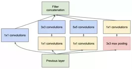
Next, let’s look at the basic structure of the Inception Module, which has four branches: the first branch performs 1×1 convolutions on the input, which is an important structure proposed in NIN. The 1×1 convolution is an excellent structure that can organize information across channels, enhancing the network’s expressive ability while allowing for dimensionality increase and decrease of output channels.

All four branches of the Inception Module utilize 1×1 convolutions for low-cost (computational load is much smaller than 3×3) cross-channel feature transformations.

The second branch first uses a 1×1 convolution, then connects to a 3×3 convolution, effectively performing two feature transformations. The third branch is similar, first using a 1×1 convolution, then connecting to a 5×5 convolution. The last branch performs a 3×3 max pooling followed by a 1×1 convolution.

The four branches of the Inception Module are finally merged through an aggregation operation (aggregating in the output channel dimension).

At the same time, Google Inception Net is a family of models, including:

• The Inception V1 proposed in the September 2014 paper “Going Deeper with Convolutions” (top-5 error rate 6.67%).

• The Inception V2 proposed in the February 2015 paper “Batch Normalization: Accelerating Deep Network Training by Reducing Internal Covariate Shift” (top-5 error rate 4.8%).

• The Inception V3 proposed in the December 2015 paper “Rethinking the Inception Architecture for Computer Vision” (top-5 error rate 3.5%).

• The Inception V4 proposed in the February 2016 paper “Inception-v4, Inception-ResNet and the Impact of Residual Connections on Learning” (top-5 error rate 3.08%).

Inception V2 learned from VGGNet, replacing large 5×5 convolutions with two 3×3 convolutions (to reduce parameter count and mitigate overfitting) and introduced the famous Batch Normalization (BN) method. BN is a very effective regularization method that can significantly speed up the training of large convolutional networks and greatly improve classification accuracy after convergence.

When BN is applied to a certain layer of a neural network, it standardizes the internal data of each mini-batch, normalizing the output to a normal distribution N(0,1), which reduces Internal Covariate Shift (the change in distribution of internal neurons).

The BN paper pointed out that traditional deep neural networks face difficulties during training due to changing input distributions at each layer, forcing us to use a very small learning rate to address this issue. However, after applying BN to each layer, we can effectively solve this problem, allowing the learning rate to be increased significantly, achieving the previous accuracy with only 1/14 of the iterations, greatly shortening training time.

After reaching previous accuracy, training can continue, ultimately achieving performance far exceeding that of the Inception V1 model—top-5 error rate of 4.8%, already surpassing human-level performance. Since BN also serves as a regularization method, it can reduce or eliminate the need for Dropout, simplifying the network structure.

ResNet (Residual Neural Network) was proposed by Kaiming He and three other researchers from Microsoft Research, successfully training a 152-layer deep neural network using Residual Units, winning the championship in the ILSVRC 2015 competition with a top-5 error rate of 3.57%, while having a lower parameter count than VGGNet, achieving outstanding results.

The structure of ResNet can rapidly accelerate the training of ultra-deep neural networks, significantly improving model accuracy.

The initial inspiration for ResNet arose from the issue of degradation: as the depth of neural networks increases, accuracy initially rises, then saturates, and further increases in depth lead to declining accuracy.

This is not a problem of overfitting, as the error increases not only on the test set but also on the training set itself. Assuming a relatively shallow network achieves saturated accuracy, adding several identity mapping layers should not increase the error, meaning deeper networks should not lead to increased training set errors.

The idea of using identity mappings to directly pass the output of the previous layer to subsequent layers is the inspiration behind ResNet. Assuming the input of a segment of the neural network is x, and the expected output is H(x), if we directly pass input x to the output as the initial result, then the target we need to learn is F(x) = H(x) – x.

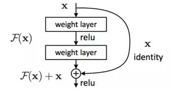
This is a residual learning unit (Residual Unit) of ResNet, which effectively changes the learning target from learning a complete output H(x) to just learning the difference between the output and the input, H(x) – x, which is the residual.

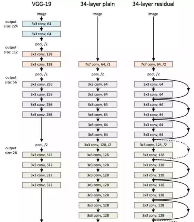
The figure shows a comparison of VGGNet-19, a 34-layer ordinary convolutional network, and a 34-layer ResNet network. It can be seen that the main difference between a standard directly connected convolutional neural network and ResNet is that ResNet has many bypass branches connecting inputs directly to later layers, allowing those layers to learn the residuals directly. This structure is also known as shortcut or skip connections.

Traditional convolutional or fully connected layers often experience information loss or degradation during information transfer. ResNet partially addresses this issue by directly passing input information to output, preserving the integrity of information, allowing the entire network to only learn the differences between input and output, simplifying the learning target and difficulty.

The figure shows the network configurations of ResNet at different depths, where the basic structure is quite similar, consisting of the previously mentioned stacked two-layer and three-layer residual learning units.

After adopting ResNet’s structure, the phenomenon of increasing training set errors with increasing depth has been eliminated; the training error of ResNet decreases as the depth increases, and its performance on the test set also improves.

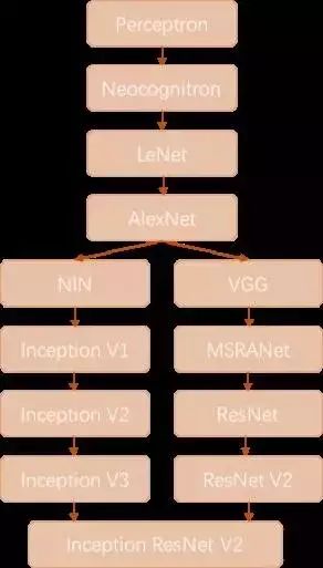
This concludes the introduction of the four classic convolutions: AlexNet, VGGNet, Inception Net, and ResNet. Below we briefly summarize. We will review the history of convolutional neural networks; the figure roughly outlines the development direction of convolutional neural networks over the past few decades.

The Perceptron was proposed in 1957 by Frank Rosenblatt, and it is not only the ancestor of convolutional networks but also of neural networks. The Neocognitron is a multi-layered neural network proposed by Japanese scientist Kunihiko Fukushima in the 1980s, which possesses a degree of visual cognitive function and directly inspired later convolutional neural networks.

LeNet-5 was proposed by the father of CNN, Yann LeCun, in 1997, which first introduced the multi-layered convolutional structure capable of effectively recognizing handwritten digits. It can be seen that the first three technological breakthroughs in convolutional neural networks were spaced apart by a significant duration, with more than a decade often passing before a theoretical innovation emerged.

Then, in 2012, Hinton’s student Alex won the championship of the ILSVRC 2012 competition with an 8-layer deep convolutional neural network, instantly igniting a surge of research in convolutional neural networks. AlexNet successfully applied new technologies such as ReLU activation functions, Dropout, max pooling, LRN layers, and GPU acceleration, inspiring further technological innovations, and research into convolutional neural networks entered a fast lane.

After AlexNet, the development of convolutional neural networks can be divided into two categories: one focused on structural improvements and adjustments (the left branch in Figure 6-18), and the other on increasing network depth (the right branch in Figure 18).

In 2013, Professor Yanshuicheng’s work on Network in Network was first published, optimizing the structure of convolutional neural networks and promoting the 1×1 convolution structure. In the work of improving convolutional network structures, subsequent contributors include Google’s Inception Net V1 in 2014, which proposed the Inception Module, an efficient convolutional network structure that can be stacked repeatedly and won the championship in that year’s ILSVRC competition.

In early 2015, Inception V2 proposed Batch Normalization, greatly accelerating the training process and enhancing network performance. The end of 2015 saw Inception V3 continue optimizing the network structure, introducing the idea of Factorization in Small Convolutions, decomposing large convolutions into multiple small convolutions or even one-dimensional convolutions.

On the right branch, many research efforts focused on deepening network layers. In 2014, the runner-up VGGNet utilized 3×3 convolutions throughout, successfully training a network with a depth of 19 layers, while the third-place MSRA-Net also employed a very deep network.

In 2015, Microsoft’s ResNet successfully trained a 152-layer deep network, winning the championship in that year’s ILSVRC competition, with a top-5 error rate reduced to 3.46%.

We can see that since AlexNet was proposed in 2012, the research and development in the field of deep learning has progressed extremely rapidly, with new technologies emerging almost every year or even every few months. New technologies are often accompanied by new network structures and methods for training deeper networks, continually setting new accuracy records in image recognition and other fields.

The technology of CNNs is evolving rapidly, with the undeniable driving force being the availability of faster GPU computing resources for experimentation and very convenient open-source tools (such as TensorFlow) that allow researchers to explore and experiment rapidly. Previously, researchers without the programming skills of someone like Alex, who could implement cuda-convnet, might not have been able to design CNNs or conduct experiments quickly.

Now with TensorFlow, researchers and developers can easily and quickly design neural network structures for research, testing, deployment, and practical application.

Q1: What is the learning path for TensorFlow?

Huang Wenjian: To quickly get started, you can combine the MNIST dataset and try MLP and CNN for image classification, and then attempt to implement an AutoEncoder on MNIST. After that, you can learn TensorBoard, which is a very convenient visualization tool. Following this, master advanced CNNs, RNNs, and reinforcement learning training methods. If interested, you can also learn about single-machine multi-GPU parallel computing and multi-machine multi-GPU distributed training. Currently, TensorFlow has also introduced many components, such as TF.Learn, Slim, XLA, Fold, etc., for targeted exploration based on needs.

Q2: What are the main advantages of TensorFlow compared to other mainstream deep learning tools like Caffe and Mxnet? What are the future development trends for TensorFlow?

Huang Wenjian: Caffe is a classic older framework, but its drawback lies in using configuration files to define network structures, making network debugging inconvenient. It has a layer-based construction method, stacking networks layer by layer, which is not convenient for representing more flexible graph structures, and its distributed capabilities are also not well-developed.

MXnet is a framework developed by Chinese authors, mainly Tianqi Chen and Mu Li. MXNet is very flexible, supports various programming paradigms, and has excellent distributed performance, with many front-end language bindings. However, its development team is small, and the stability of the framework’s code quality is not as good as TensorFlow. Moreover, it lacks comprehensive documentation and resources.

TensorFlow is a framework vigorously developed by Google, with about 100-200 full-time engineers collaborating, ensuring product-level code quality, stability, and high reliability, making it suitable for production environments. Its computational graph definition mode is also very flexible, allowing for various debugging methods. Currently, most new papers and research are implemented using TensorFlow, with many available model codes.

In the TensorFlow Models repository, there are also many reliable open-source model implementations, such as SyntaxNet and TextSum. TensorFlow has also garnered the most stars on GitHub among machine learning libraries, ranking first, essentially equal to the sum of the second to tenth places.

Q3: How does TensorFlow perform in the text domain?

Huang Wenjian: For text analysis and processing, RNNs are mainly used, with CNNs used in fewer cases. Both of these networks are well-supported and comprehensive in TensorFlow. Additionally, the newly introduced TensorFlow Fold supports dynamic batch inputs, significantly speeding up dynamic RNN structures.

Q4: How do I choose the number of layers and neurons for a network?

Huang Wenjian: The number of layers and neurons in deep learning is always a very empirical issue. In TensorFlow, you can use TensorBoard to observe train loss and test loss. If the train loss decreases slowly and the test loss does not increase, you can increase model fitting capacity, i.e., deepen the network and increase the number of neurons. If the train loss is hard to decrease and the test loss starts to rebound, you should control model capacity, ensuring the number of layers and neurons does not become too large while using various methods to alleviate overfitting, such as dropout and batch normalization.

If the train loss is hard to decrease and the test loss starts to rebound, you should control model capacity, ensuring the number of layers and neurons does not become too large while using various methods to alleviate overfitting, such as dropout and batch normalization.

Q5: How can TensorFlow be applied in practical projects, and what should the data conversion and structure be like?

Huang Wenjian: TensorFlow’s format can use numpy arrays, and input data is converted to tensors through placeholders, which are multi-dimensional array formats, the core data format of TensorFlow.

For data with spatial correlation and temporal management, CNNs and RNNs should be connected for processing, while other types of data should use MLP.

Q6: What are the suitable scenarios for RNNs and CNNs?

Huang Wenjian: CNNs are suitable for scenarios where spatial and temporal correlations exist, such as image classification, text classification, and time series classification.

RNNs are mainly suitable for scenarios with temporal correlations and are sensitive to the order of time, making them suitable for text classification and language modeling.

Q7: I am a Java programmer with 5 years of work experience. How can I better learn TensorFlow?

Huang Wenjian: The mainstream interface for TensorFlow is Python, but a Java interface has also been introduced. If you are interested, you can start with the Java interface, but debugging might be inconvenient since it is not a scripting language; later, you can learn the Python interface.

Q8: What is your view on the relationship between Keras and TensorFlow? Should Keras, as a higher-level library, be learned together with TF, or is it better to recommend the lower-level TF as an entry point for deep learning frameworks?

Huang Wenjian: Keras has been integrated into TensorFlow; it can now be considered a component of TF. It is recommended to first learn TensorFlow and grasp some underlying mechanisms. Later, when you need to quickly build large neural network experiments, you can learn Keras. After learning TensorFlow, Keras will be very simple.