This articleis approximately 5200 words, recommended reading time is10+minutesWe know that, to some extent, the deeper the network, the more parameters it has, and the more complex the model, the better its final performance.The compression algorithm for neural networks aims to transform a large and complex pre-trained model into a streamlined smaller model.Based on the degree of destruction to the network structure during the compression process, we categorize modelcompression techniques into “frontend compression” and “backend compression”.
Frontend compression refers to compression techniques that do not alter the original network structure, mainly including knowledge distillation, lightweight networks (compact model structure design), and pruning at the filter layer level (structured pruning);
Backend compression includes low-rank approximation, unrestricted pruning (unstructured pruning/sparsity), parameter quantization, and binary networks, aiming to minimize model size, which can significantly alter the original network structure.
Summary: Frontend compression hardly changes the original network structure (only reduces the number of layers or filters), while backend compression makes irreversible significant changes to the network structure, leading to incompatibility with existing deep learning libraries or even hardware devices, resulting in high maintenance costs.
1. Low-Rank Approximation
Simply put, the weight matrix of convolutional neural networks is often dense and large, resulting in high computational overhead. One approach is to use low-rank approximation techniques to reconstruct this dense matrix from several smaller matrices, which is classified as low-rank approximation algorithms.Generally, the rank of a row echelon matrix equals its “number of steps” – the number of non-zero rows.The principle of low-rank approximation algorithms in reducing computational overhead is as follows:Based on the above idea, Sindhwani et al. proposed an algorithm using structured matrices for low-rank decomposition; specific principles can be referenced in their paper. Another more straightforward method is to use matrix decomposition to reduce the parameters of the weight matrix, such as the method proposed by Denton et al., which uses Singular Value Decomposition (SVD) to reconstruct the weights of the fully connected layer.
1.1 Summary
Low-rank approximation algorithms have achieved good results on medium and small network models, but their hyperparameter count scales linearly with the number of network layers. As the number of layers increases and model complexity rises, the search space expands dramatically. Currently, this is mainly studied in academia with limited industrial application.
2. Pruning and Sparse Constraints
Given a pre-trained network model, common pruning algorithms generally follow these steps:
Assess the importance of neurons;
Remove some unimportant neurons, which is more straightforward and flexible than the previous step;
Fine-tune the network, as pruning inevitably affects the network’s accuracy; to prevent excessive damage to classification performance, the pruned model must be fine-tuned. For large-scale image datasets (like ImageNet), fine-tuning can consume significant computational resources, so the extent of fine-tuning requires careful consideration;
Return to the first step and iterate for the next round of pruning.
Based on this iterative pruning framework, different scholars have proposed various methods. Han et al. proposed first removing all weight connections below a certain threshold, followed by fine-tuning the pruned network to complete parameter updates. A drawback of this method is that the pruned network is unstructured, meaning the removed network connections lack continuity in distribution, leading to frequent switching between CPU cache and memory, thereby limiting actual acceleration effects.Based on this method, some researchers have attempted to elevate the pruning granularity to the level of entire filters, i.e., discarding entire filters. However, measuring the importance of filters poses a challenge. One strategy is based on statistical measures of filter weights, such as calculating the L1 or L2 values of each filter and using the corresponding value size as a standard for measuring importance.Using sparse constraints for network pruning is also a research direction, where the idea is to incorporate a sparse regularization term for weights into the network’s optimization objective, causing some weights to approach zero during training, and these zeros become the targets for pruning.
2.1 Summary
Overall, pruning is an effective general compression technique to reduce model complexity, with its key challenge being how to measure the importance of individual weights to the overall model. The pruning operation minimally damages the network structure, and combining pruning with other backend compression techniques can achieve maximum compression of the network model. Currently, there are industrial cases using pruning methods for model compression.
3. Parameter Quantization
Compared to pruning operations, parameter quantization is a commonly used backend compression technique. “Quantization” refers to summarizing several “representatives” from weights, using these “representatives” to represent specific values of a class of weights. The “representatives” are stored in a codebook, while the original weight matrix only needs to record the index of each “representative”, thus greatly reducing storage overhead. This idea can be likened to the classic bag-of-words model. Common quantization algorithms include:
Scalar quantization.
Scalar quantization can somewhat reduce the network’s accuracy. To mitigate this drawback, many algorithms consider structured vector methods, one of which is Product Quantization (PQ); details can be referenced in their papers.
Based on the PQ method, Wu et al. designed a universal network quantization algorithm: QCNN (quantized CNN), primarily based on the idea that minimizing the reconstruction error of each layer’s network output is more effective than minimizing quantization error.
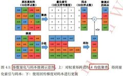
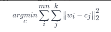
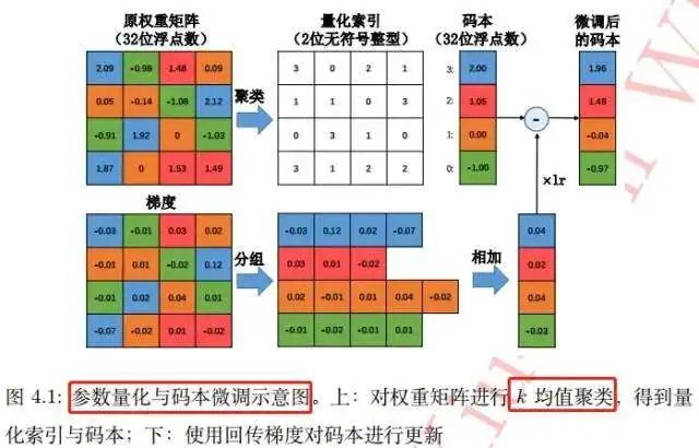
Thus, only the kk cluster centers (cjcj, scalar) need to be stored in the codebook, while the original weight matrix only needs to record the indices of their respective cluster centers in the codebook. If we disregard the storage overhead of the codebook, this algorithm can reduce storage space to log2(k)/32. Scalar quantization based on kk-means algorithm is very effective in many applications. The diagram below illustrates the parameter quantization and codebook fine-tuning process:These three types of clustering-based parameter quantization algorithms fundamentally aim to map multiple weights to the same value, thereby achieving weight sharing and reducing storage overhead.
3.1 Summary
Parameter quantization is a commonly used backend compression technique that can achieve a significant reduction in model size with minimal performance loss. However, a drawback is that the quantized network is “fixed”, making any changes difficult, and this method has poor universality, requiring specific deep learning libraries to run the network.Here, weight parameters are converted from floating-point to fixed-point, binarization, etc., which are methods attempting to avoid the time-consuming floating-point calculations. These methods can speed up computation while reducing memory and storage space usage, ensuring that model accuracy loss remains within acceptable limits; thus, their application is of practical value.For more knowledge on parameter quantization, please refer to this GitHub repository:https://github.com/Ewenwan/MVision/blob/master/CNN/Deep_Compression/quantization/readme.md
4. Binary Networks
1. Binary networks can be viewed as an extreme case of quantization methods: all weight parameters can only take values of ±1, meaning that 1 bit is used to store weights and features. In a standard neural network, a parameter is represented bya single-precision floating-point number, and the binarization of parameters can reduce storage overhead to 1/32 of the original.2. Binary neural networks have gained significant attention and development in recent years due to their high model compression rates and advantages in computational speed during forward propagation, becoming a very popular research direction in neural network modeling. However, the first paper to truly binarize both weight values and activation function values in neural networks was published by Courbariaux et al. in 2016, titled “BinaryNet: Training Deep Neural Networks with Weights and Activations Constrained to +1 or -1”. This paper first provided methods for binarizing networks and training binary neural networks.3. A typical module of CNN networks consists of convolution (Conv) -> batch normalization (BNorm) -> activation (Activ) -> pooling (Pool). For XOR neural networks, the designed module is composed of batch normalization (BNorm) -> binarized activation (BinActiv) -> binarized convolution (BinConv) -> pooling (Pool). This approach ensures that after batch normalization, the input has a mean of 0, then undergoes binarized activation to ensure data is either -1 or +1, followed by binarized convolution, which minimizes the loss of feature information. The definition instance code for the binarized residual network structure is as follows:<span>def residual_unit(data, num_filter, stride, dim_match, num_bits=1):</span><span> """Residual Block Definition"""</span><span> bnAct1 = bnn.BatchNorm(data=data, num_bits=num_bits)</span><span> conv1 = bnn.Convolution(data=bnAct1, num_filter=num_filter, kernel=(3, 3), stride=stride, pad=(1, 1))</span><span> convBn1 = bnn.BatchNorm(data=conv1, num_bits=num_bits)</span><span> conv2 = bnn.Convolution(data=convBn1, num_filter=num_filter, kernel=(3, 3), stride=(1, 1), pad=(1, 1))</span><span> if dim_match:</span><span> shortcut = data</span><span> else:</span><span> shortcut = bnn.Convolution(data=bnAct1, num_filter=num_filter, kernel=(3, 3), stride=stride, pad=(1, 1))</span><span> return conv2 + shortcut</span>
4.1 Gradient Descent in Binary Networks
Current neural networks are almost all trained based on gradient descent algorithms, but the weights of binary networks are only ±1, making it impossible to directly compute gradient information or perform weight updates. To address this issue, Courbariaux et al. proposed the binary connect algorithm, which combines single precision with binary to train binary neural networks. The process is as follows:1. Initialize weights as floating-point.2. Forward Pass:
Use a deterministic method (sign(x) function) to quantize weights to +1/-1, with 0 as the threshold.
Use the quantized weights (only +1/-1) to compute the forward pass, performing convolution operations with binary weights and inputs (which effectively only involves addition) to obtain the convolution layer output.
3. Backward Pass:
Update the gradient to the floating-point weights (calculating the corresponding gradient based on the relaxed sign function and updating the single precision weights based on that gradient value).
End of training: Permanently convert weights to +1/-1 for inference use.
4.2 Two Problems
Network binarization needs to address two issues: how to binarize weights and how to compute gradients of binary weights.1. How to binarize weights?Weight binarization generally has two options:
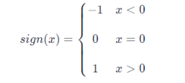
Directly binarize based on the sign of the weights: xb=sign(x). The sign function sign(x) is defined as follows:
Random binarization, i.e., for each weight, take ±1 with a certain probability.
2. How to compute gradients of binary weights?The gradient of binary weights is 0, making parameter updates impossible. To resolve this issue, the sign function needs to be relaxed, using Htanh(x)=max(−1,min(1,x)) instead of sign(x). When x is in the interval [-1,1], the gradient value is 1; otherwise, the gradient is 0.
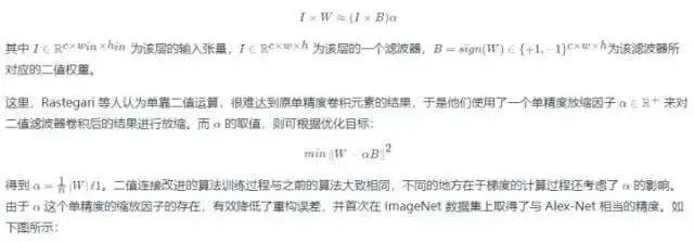
4.3 Improvements to the Binary Connect Algorithm
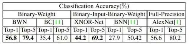
The previous binary connect algorithm only binarized weights, but the intermediate output values of the network remained single precision. Rastegari et al. improved this by proposing an algorithm that uses a single precision diagonal matrix multiplied by a binary matrix to approximate the original matrix to enhance the classification performance of binary networks, compensating for their accuracy weaknesses. This algorithm decomposes the original convolution operation into the following process:It can be seen that the accuracy of weight binarized neural networks (BWN) is almost the same as that of full precision neural networks, but compared to XOR neural networks (XNOR-Net), there is a loss of over 10% in both Top-1 and Top-5.Compared to weight binarized neural networks, XOR neural networks also convert the network inputs to binary values, so the multiplication and accumulation operations in XOR neural networks are replaced by bitwise XOR and popcount.
4.4 Design Considerations for Binary Networks
Avoid using Convolution with kernel=(1,1) (including ResNet bottlenecks): Since all weights in binary networks are 1 bit, using a 1×1 size will significantly reduce expressiveness.
Increasing the number of channels + increasing activation bits should be coordinated: If only the number of channels is increased, the feature map may waste model capacity due to low bit count. The reverse is also true.
It is recommended to use 4 bits or fewer for activation bits; higher values yield diminishing returns in accuracy while significantly increasing inference computation.
5. Knowledge Distillation
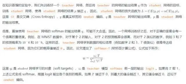
This article only briefly introduces the pioneering work in this field – “Distilling the Knowledge in a Neural Network”, which is the method of distilling “logits”, followed by papers that distill “features”. For a deeper understanding, a Chinese blog can refer to this article – What is Knowledge Distillation? An Introductory Essay.Knowledge distillation is a form of transfer learning, simply put, it involves training a large model (teacher) and a small model (student), transferring the knowledge learned from the large and complex model to the streamlined small model through certain technical means, enabling the small model to achieve performance close to that of the large model.Therefore, the loss function of the student model ultimately consists of two parts:
The first part is the cross-entropy (cross entropy) formed by the predictions of the small model and the “soft labels” from the large model;
The second part is the cross-entropy between the prediction results and the standard class labels.
The importance of these two loss functions can be adjusted through certain weights. In practical applications, the value of T affects the final result; generally, a larger T can achieve higher accuracy. T (the distillation temperature parameter) is a type of hyperparameter in knowledge distillation model training. T is an adjustable hyperparameter; the larger the T, the softer the probability distribution (as described in the paper), and the smoother the curve, which effectively adds perturbation during the transfer learning process, enhancing the efficiency of the student network in learning and improving its generalization ability. This is essentially a strategy to suppress overfitting. The entire process of knowledge distillation is illustrated in the diagram below:The actual model structure of the student model is the same as that of the small model, but the loss function includes two parts. The MXNet code example of knowledge distillation in classification networks is as follows:<span># -*-coding-*- : utf-8 </span><span>"""</span><span>This program does not provide specific model structure code; it mainly presents the softmax loss calculation part of knowledge distillation.</span><span>"""</span><span>import mxnet as mx</span><span>def get_symbol(data, class_labels, resnet_layer_num,Temperature,mimic_weight,num_classes=2):</span><span> backbone = StudentBackbone(data) # Backbone is the classification network backbone class</span><span> flatten = mx.symbol.Flatten(data=conv1, name="flatten")</span><span> fc_class_score_s = mx.symbol.FullyConnected(data=flatten, num_hidden=num_classes, name='fc_class_score')</span><span> softmax1 = mx.symbol.SoftmaxOutput(data=fc_class_score_s, label=class_labels, name='softmax_hard')</span><span> import symbol_resnet # Teacher model</span><span> fc_class_score_t = symbol_resnet.get_symbol(net_depth=resnet_layer_num, num_class=num_classes, data=data)</span><span> s_input_for_softmax=fc_class_score_s/Temperature</span><span> t_input_for_softmax=fc_class_score_t/Temperature</span><span> t_soft_labels=mx.symbol.softmax(t_input_for_softmax, name='teacher_soft_labels')</span><span> softmax2 = mx.symbol.SoftmaxOutput(data=s_input_for_softmax, label=t_soft_labels, name='softmax_soft',grad_scale=mimic_weight)</span><span> group=mx.symbol.Group([softmax1,softmax2])</span><span> group.save('group2-symbol.json')</span><span> return group</span>TensorFlow code example is as follows:<span><span># One-hot encoding of class labels</span></span><span>one_hot = tf.one_hot(y, n_classes,1.0,0.0) <span># n_classes is the total number of classes, n is the class label</span></span><span><span># one_hot = tf.cast(one_hot_int, tf.float32)</span></span><span>teacher_tau = tf.scalar_mul(1.0/args.tau, teacher) <span># teacher is the output tensor of the teacher model, tau is the temperature coefficient T</span></span><span>student_tau = tf.scalar_mul(1.0/args.tau, student) <span># The logits tensor of the student model is at temperature coefficient T</span></span><span>objective1 = tf.nn.sigmoid_cross_entropy_with_logits(student_tau, one_hot)</span><span>objective2 = tf.scalar_mul(0.5, tf.square(student_tau-teacher_tau))</span><span><span>"""</span><span>"""</span></span><span>student model's final loss function consists of two parts:</span><span>The first part is the cross-entropy formed by the predictions of the small model and the "soft labels" from the large model;</span><span>The second part is the cross-entropy between the prediction results and the standard class labels.</span><span><span>"""</span><span>"""</span></span><span>tf_loss = (args.lamda*tf.reduce_sum(objective1) + (1-args.lamda)*tf.reduce_sum(objective2))/batch_size</span>The tf.scalar_mul function is a scalar scaling function for tf tensors. Typically, the value of T ranges from 1 to 20; here I referred to open-source code with a value of 3. I found that in open-source code, the training of the student model is sometimes done together with the teacher model, and sometimes the student model is trained directly under the guidance of the teacher model.
6. Shallow / Lightweight Networks
Shallow networks: Achieve approximation of complex model performance by designing a shallower (fewer layers) and more compact structure, but the expressive ability of shallow networks is hard to match that of deep networks. Therefore, the limitation of this design method is that it can only be applied to relatively simple problems, such as tasks with fewer categories in classification problems.Lightweight networks: Using lightweight network structures such as MobileNetV2, ShuffleNetV2, etc., as the backbone model can significantly reduce the number of model parameters.
References:
Knowledge Distillation in Neural Network Model Compression and Acceleration