In recent years, artificial intelligence has developed rapidly, gradually penetrating various industries and fields. More and more people are learning AI-related technologies. To help beginners quickly grasp the basic principles of AI, Professor Ma Shaoping, Vice Chairman of CAAI, has written an introductory book titled “How Computers Achieve Intelligence.” Through the new popular science column “Learn AI with Me,” we will share chapters from the book along with several explanatory videos to help you understand the corresponding AI knowledge points.
Author Profile

Ma Shaoping
Vice Chairman of CAAI
Executive Vice Dean and Professor at Tsinghua University’s Institute of Intelligent Computing
CAAI Fellow
Personal Profile:
Former Vice Chairman of CAAI. PhD supervisor, Director of the Intelligent Information Retrieval Research Center at Tsinghua University’s Institute of Artificial Intelligence, focusing on research in intelligent information processing, particularly in information retrieval, achieving a series of research results. The information retrieval group he leads has ranked first in the Web and Information Retrieval direction on CSRankings for nearly a decade. He has undertaken multiple projects under the “973 Program,” “863 Program,” and the National Natural Science Foundation.
Video Version: How Neural Networks Are Implemented (Part 3 Upper)
Video Version: How Neural Networks Are Implemented (Part 3 Lower)
Section 3: How Neural Networks Are Trained
Xiao Ming heard Dr. Ai introduce that a neural network can recognize different things by training on different data. He was amazed and curiously asked Dr. Ai: “Dr. Ai, could you explain how neural networks are trained?”
Dr. Ai appreciated Xiao Ming’s curiosity and said: “Sure, let’s begin to introduce how neural networks are trained. Xiao Ming, can you tell me how you recognize animals?”
Xiao Ming replied: “When I was a child, every time I saw a small animal, my mom would tell me what kind of animal it was. After seeing many, I gradually recognized these small animals. Is that how neural networks recognize animals too?”
Dr. Ai said: “Yes, neural networks also recognize animals through samples. Humans are smart; after seeing a cat once, they might recognize it as a cat next time. However, neural networks are a bit slow and need a large number of samples to be trained well. For example, if we want to build a neural network that can recognize both cats and dogs, we first need to collect a large number of photos of cats and dogs, including different breeds, sizes, and poses, and label which photos are cats and which are dogs, just like your mom tells you which is a cat and which is a dog. This is the first step in training a neural network; the more data, the better. In fact, we humans sometimes do the same thing; the saying ‘familiarity breeds understanding’ reflects this idea of broad exposure.
Once the data is prepared, the next step is training. Training involves adjusting the weights of the neural network so that when a cat photo is input, the output corresponding to the cat is close to 1, and the output for the dog is close to 0, while when a dog photo is input, the output for the dog is close to 1 and the output for the cat is close to 0.
Xiao Ming: “How is this achieved?”
Dr. Ai then asked Xiao Ming: “Do you take a bath every day? How do you adjust the temperature of the water heater?”
Xiao Ming looked at Dr. Ai in confusion, thinking, “I asked how neural networks are trained; why is he talking about bathing?” But since Dr. Ai asked, he had to answer: “It’s easy! The water heater has two knobs, one for hot water and one for cold water. If the water feels hot, I turn up the cold water; if it feels cold, I turn up the hot water.”
Dr. Ai asked again: “When the water feels hot, you can also turn down the hot water, and when it feels cold, you can turn down the cold water, right?”
Xiao Ming thought about it and replied: “Yes, there are different ways to adjust, and which one to adjust might depend on the amount of water. For example, if the water feels hot but the amount is large, I can reduce the hot water; if the amount is small, I can increase the cold water. In short, I need to adjust based on both water temperature and water amount.”
Dr. Ai saw that Xiao Ming finally got to the point. After confirming his statement, he added: “There is also the issue of adjustment size. If the difference between the water temperature and your ideal temperature is large, you can adjust the valve more significantly; if the difference is small, you adjust it less. After multiple adjustments, you can achieve a more ideal water temperature and amount.”
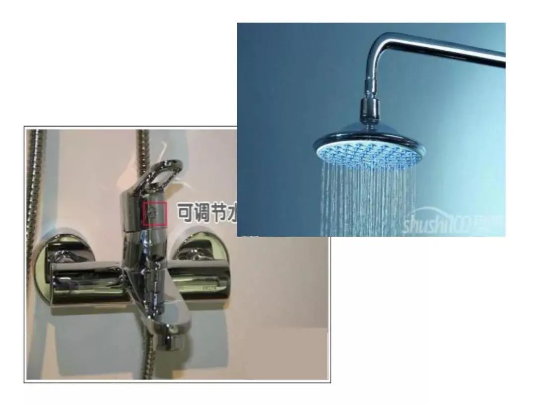
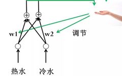
Figure 1.9 Water Heater Adjustment Diagram
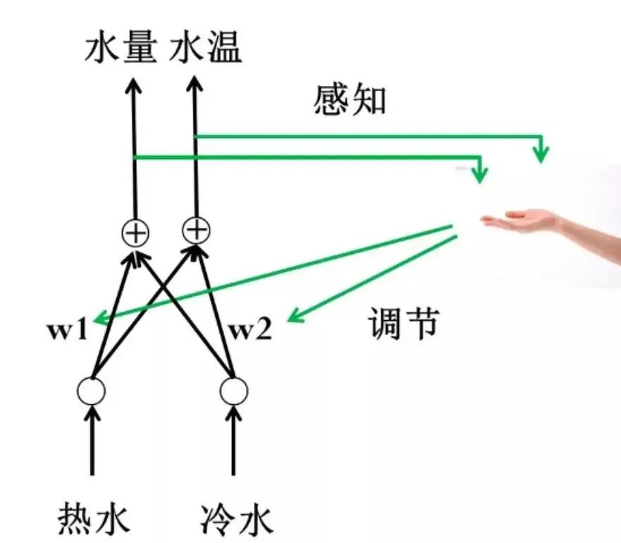
Figure 1.10 The Water Heater Can Be Represented as a Neural Network
Dr. Ai said to Xiao Ming: “We can abstract the water heater as shown in Figure 1.10. Do you see that this is a neural network?”
Xiao Ming tapped his little head and said: “I finally understand! This is indeed a neural network. The two inputs are hot water and cold water, the sizes of the hot and cold water valves correspond to the weights, and the point where the hot and cold water converge is equivalent to a weighted sum. Finally, the water coming out of the showerhead corresponds to the two outputs: one for water temperature and one for water amount.”
So, is adjusting the hot and cold water valves equivalent to training? Xiao Ming tilted his head and asked.
Dr. Ai replied: “Exactly. When adjusting the water valves, you can adjust them to a larger or smaller extent, which is the direction of adjustment. You can also adjust a lot at once or just a little, which is the size of the adjustment. Additionally, you can decide which valve to adjust or whether to adjust both, but the size and direction might differ.”
Xiao Ming exclaimed: “I didn’t expect that such a simple task of adjusting the bathwater could have so much knowledge behind it. So how is this idea applied to training neural networks?”
Dr. Ai said: “Before we discuss how to train a neural network, we should first talk about how to evaluate whether a neural network has been trained well. This is closely related to training a neural network. In the previous example with the water heater, under what circumstances would you consider the water heater to be adjusted well?”
Xiao Ming replied: “If I think the water temperature and amount are about what I want, I would consider it adjusted well.”
Dr. Ai said: “Exactly. But for a computer, what does ‘about’ mean? There needs to be a measurement standard. For example, we can use  to represent the desired water temperature,
  to represent the actual water temperature,
  to represent the desired water amount, and
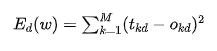
  to represent the actual water amount. This way, we can use the error between the desired value and the actual value to measure whether they are “about the same.” When the error is small, we consider that the water temperature and amount have been adjusted well. However, since the error can be positive (when the actual value is less than the desired value) or negative (when the actual value is greater than the desired value), it is inconvenient to use, so we often use the “sum of squared errors” as the measurement standard. It is expressed as follows:
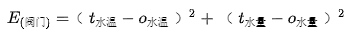
Where E is a function of the valve sizes. By appropriately adjusting the sizes of the cold and hot water valves, we can make E obtain a relatively small value. When E is small, we consider that the water heater is adjusted well. Here, the “valve” corresponds to the weights w of the neural network.
For a neural network, we assume there are M outputs. For an input sample d, we use 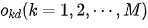 to represent the M actual output values of the network. The target output values corresponding to these outputs are
 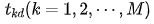 . The sum of squared errors for the neural network output for this sample d can be expressed as:
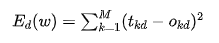
This is the sum of squared errors for a single sample d. If it is for all samples, we just need to add the output sum of squared errors for all samples together, which we denote as E(w):
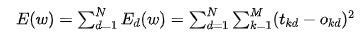
Here, N represents the total number of samples. We usually call E(w) the loss function; of course, there are other forms of loss functions, and the sum of squared errors is just one of them. Here, w is a vector composed of all the weights of the neural network. The training problem of the neural network is to find suitable weights that minimize the loss function.
Xiao Ming looked at the formula and asked in confusion: “Dr. Ai, how can we solve so many weights in a neural network?”
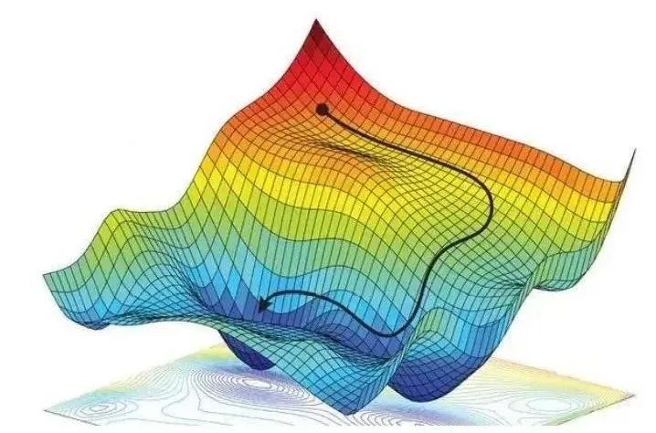
Dr. Ai replied: “This is indeed a complex optimization problem. Let’s start with a simple example. Suppose the function f(θ) is shown in Figure 1.11, this function has only one variable θ. How do we calculate its minimum value?”
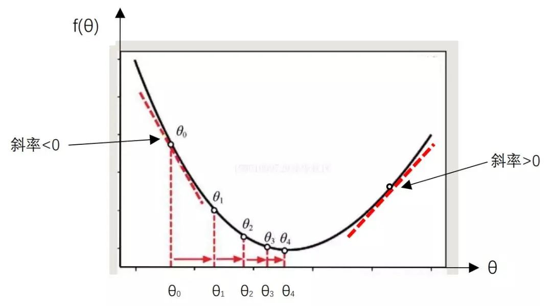
Figure 1.11 Illustration of Minimum Value Calculation
The basic idea is to start by randomly selecting a value  as
as  , then modify
  to get
  , and then modify
  to get
  . By iterating this way,
  gradually approaches the minimum value.
Assuming the current value is  , the modification amount for
  is
is  . Thus:
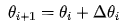
How to calculate  ? Two points need to be determined: one is the size of the modification, and the other is the direction of modification, i.e., whether to increase or decrease.
Xiao Ming, look at Figure 1.11. The areas far from the minimum value are steep, while those near the minimum value are flat. Therefore, without any other information, we have reason to believe that the steeper the area, the farther it is from the minimum value. In such a case, the modification amount for  should be larger, while in flatter areas, the modification amount should be smaller to avoid overshooting the minimum value. Therefore, the size of the modification amount, which is the absolute value of
  , should be related to the steepness of the area; the steeper it is, the larger the modification amount should be, and the flatter it is, the smaller the modification amount should be.
Xiao Ming, can you tell me how to measure the steepness of a curve at a certain point?
Xiao Ming quickly replied: “Dr. Ai, we learned about the derivative of a function. The derivative at a certain point is the slope of the tangent line to the curve at that point, and the size of the slope directly reflects the steepness at that point. Can we use the derivative value as a measure of the steepness of the curve at a certain point?”
Dr. Ai said: “Xiao Ming, you are a thoughtful child! The derivative indeed reflects the steepness of the curve at a certain point. The next question is how to determine the modification direction of θ, whether to increase or decrease θ.”
Dr. Ai pointed to Figure 1.11 and asked Xiao Ming: “What characteristics do the derivatives have on both sides of the minimum value?”
Xiao Ming thought for a moment about what he learned in advanced mathematics and replied: “As we mentioned earlier, the derivative at a certain point is the slope of the tangent line at that point. Looking at the left side of Figure 1.11, the tangent line slopes downward, and its slope is a negative number less than 0. On the right side of Figure 1.11, the tangent line slopes upward, and its slope is a positive number greater than 0.”
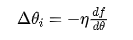
Dr. Ai continued from Xiao Ming’s words: “The derivative value on the left is negative, so θ should be increased; on the right, the derivative value is positive, so θ should be decreased. This way, θ can move closer to the point where f(θ) takes the minimum value. Therefore, the modification direction of θ is exactly opposite to the sign of the derivative value. Thus, we can modify the θi value as follows:
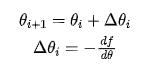
Where  represents the derivative of the function f(θ).
Xiao Ming listened to Dr. Ai’s explanation and excitedly said: “This solves the problem of finding the minimum value, right?”
Dr. Ai replied: “There is still one problem. If the derivative value is too large, it may cause the modification amount to be too large, overshooting the optimal value, resulting in oscillation as shown in Figure 1.12, which reduces the solving efficiency.
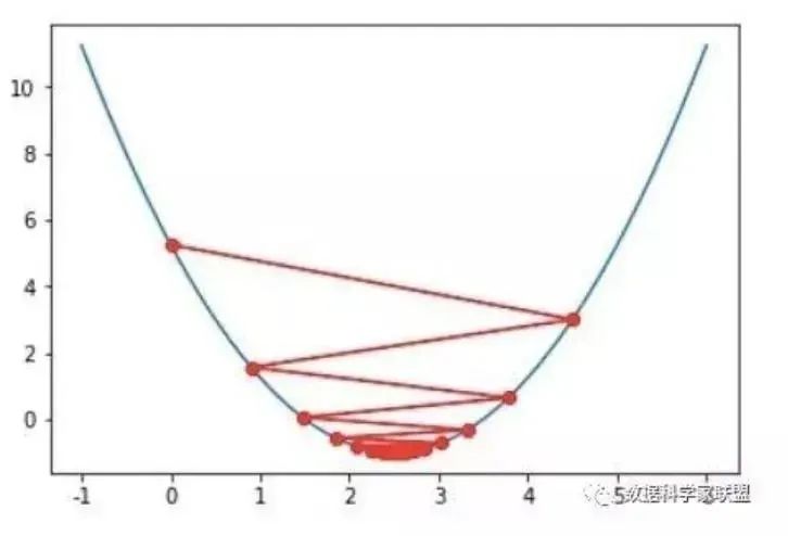
Figure 1.12 Oscillation May Occur When the Step Size Is Too Large
Xiao Ming scratched his head and asked: “What should we do then?”
Dr. Ai said: “One simple solution is to multiply the modification amount by a constant called the learning rate η, which is a positive number less than 1, making the modification amount artificially smaller. That is:
The learning rate η needs to be chosen appropriately, often determined by experience and experimentation. There are also methods for automatically selecting learning rates, even variable learning rates, which we will not discuss today. If you are interested, you can refer to related materials.
Xiao Ming asked Dr. Ai: “Is this how neural networks are trained?”
Dr. Ai said: “The basic principles are the same. Xiao Ming, do you remember the goal we want to optimize when training a neural network?”
Xiao Ming replied: “I remember! It’s to minimize the sum of squared errors, which is the minimum value of the loss function E(w) we discussed earlier.”
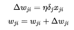
Dr. Ai said: “We can use the same method to find the minimum value of E(w). The difference is that E(w) is a multivariable function, with all weights being variables that need to be solved. The way to modify each weight is the same as the way to modify θ we discussed earlier; we just need to use partial derivatives instead of derivatives. If we denote a certain weight as wi, we update the weight using the following formula:
 as follows:
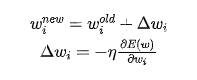
Where  ,
,  represent the values before and after modification, and
  represents the partial derivative of E(w) with respect to
  . The vector composed of all the partial derivatives with respect to
  is called the gradient, denoted as
  :
:

So, the modification for all w can be expressed using gradients as:

Here,  ,
,  ,
,  ,
,  are all vectors, and
  is a constant. Two vectors are added by adding corresponding elements, and a constant multiplied by a vector means multiplying that constant with each element of the vector, resulting in another vector.
Xiao Ming looked at the gradient symbol and asked Dr. Ai: “Dr. Ai, what is the physical meaning of the gradient here?”
Dr. Ai replied: “Just as the derivative with a single variable represents the steepness of a function curve at a certain point, the gradient reflects the steepness of a surface in multi-dimensional space at a certain point. Just like when we go down a mountain, we always choose the steepest direction from our current position. Therefore, this method of finding the minimum value of a function is also called the gradient descent algorithm.”
Xiao Ming asked again: “Dr. Ai, it seems that the main problem in training neural networks is how to calculate the gradient?”
Dr. Ai replied: “Indeed, that is the case. For neural networks, due to the many neurons in different layers, calculating the gradient is a bit complex. There are also three situations in the calculations. One is the standard gradient descent method mentioned here. In this method, all training samples are used to calculate the gradient. Generally, the training sample size is large, and calculating the output for all samples each time we update a weight can be quite intensive. Another extreme method is to calculate the gradient for each sample and then update the weight. This method is called stochastic gradient descent. Since each sample adjusts the value of w once, the calculation speed is relatively fast, and in general, a decent result can be obtained quickly. When using this method, the training samples must be randomly arranged. For example, when training a neural network to recognize cats and dogs, we cannot use all cats first and then all dogs; instead, we need to interleave cats and dogs randomly to achieve a better result. This is also where the name stochastic gradient descent algorithm comes from.
Xiao Ming: “This is a good method, but will using only one sample at a time cause problems?”
Dr. Ai: “Indeed, there are problems. The stochastic gradient descent method may decrease quickly in the early stages of training, but in the later stages, especially as it approaches the minimum value, it may not perform well. After all, the gradient is calculated based on one sample and does not represent the gradient direction for all samples. Additionally, individual bad samples, or even mislabeled samples, can have a significant impact on the results.”
At this point, Dr. Ai asked Xiao Ming: “We discussed two situations: one where all samples are used at once and one where only one sample is used. Can you think of a compromise?”
Xiao Ming tilted his head and said: “A compromise… if it’s neither all nor one, it must be using a part at a time?”
Dr. Ai happily looked at Xiao Ming and said: “Yes, a method that lies between the two is to calculate the gradient using a small batch of samples at a time and modify the weights w. This method is called mini-batch gradient descent and is currently the most commonly used method in neural network optimization.”
Xiao Ming said: “I understand these three methods, but I still don’t know how to calculate the gradient!”
Dr. Ai said: “Don’t worry, Xiao Ming; we will soon discuss how to calculate the gradient. Actually, the three methods above only differ in the number of samples used for calculations, while the method for calculating the gradient is similar. For simplicity, we will use stochastic gradient descent as an example, which can easily be extended to gradient descent or mini-batch gradient descent.”
Now let’s provide a specific algorithm description for training a neural network using stochastic gradient descent. If you want to understand how this algorithm is derived, please refer to the relevant materials.
Using the stochastic gradient descent algorithm to train a neural network aims to minimize the following expression:
Where d is a given sample, M is the number of output layer neurons,  is the desired output value for sample d, and
  is the actual output value for sample d.
For convenience, we denote the i-th input of neuron j in the neural network as  and the corresponding weight as
  . Here, neuron j may belong to the output layer or a hidden layer.
  may not necessarily be the input to the neural network; it could also be the output of the i-th neuron in the previous layer connected directly to neuron j. We derive the stochastic gradient descent algorithm as follows:
Algorithm: Stochastic Gradient Descent Algorithm:
1. Assign a small random value to all weights of the neural network, such as [-0.05, 0.05].
2. Before the stopping condition is met:
3. For each training sample:
4. Input the sample into the neural network, calculating the output of each neuron from the input layer to the output layer.
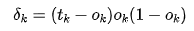
5. For the output layer neuron k, calculate the error term:
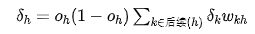
6. For the hidden layer neuron h, calculate the error term:
7. Update each weight:
In the second line of the algorithm, the stopping condition can be set as when the maximum  among all samples is less than a given value, or when the maximum
  among all samples is less than a given value, the algorithm ends.
Xiao Ming pointed at line 6 of the algorithm and asked Dr. Ai: “What does  in this formula mean?”
Dr. Ai explained: “h is a hidden layer neuron, and its output will connect to the next layer of neurons. The ‘subsequent (h)’ refers to all neurons that take h’s output as input. For a fully connected neural network, this means all neurons in the next layer where h is located.”
In the formula on line 6:
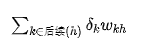 is obtained by multiplying the error term of each subsequent neuron by the weight from h to neuron k and summing them up.
After Xiao Ming understood the meaning of these symbols, he asked Dr. Ai: “Dr. Ai, this algorithm seems to start from the output layer, first calculating the  value for each neuron in the output layer. Once we have the
  values, we can update the weights of the output layer neurons. Then, using the
  values of the output layer neurons, we can calculate the
  of the previous layer neurons. This way, we can push forward layer by layer, using the
  values of the previous layer to calculate the
  values, allowing us to update the weights of all neurons. This is truly clever!”
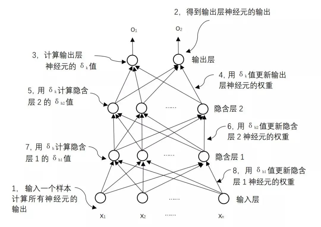
Figure 1.14 Illustration of the BP Algorithm Calculation Process
Dr. Ai said: “Xiao Ming’s analysis is very correct. When a training sample is given, we first calculate the output values of each neuron from the input to the output using the current weights. Then, we begin from the output layer to calculate the δ values for each neuron in reverse, allowing us to update the weights for each neuron. As shown in Figure 1.14, this process of calculating in reverse layer by layer is why it is called the “backpropagation algorithm,” abbreviated as BP algorithm. This algorithm is also the fundamental algorithm for training neural networks. Not only can it train fully connected neural networks, but as of now, any neural network uses this algorithm, with specific calculations varying based on the structure of the neural network.”
Dr. Ai emphasized: “The specific calculation methods in the stochastic gradient algorithm presented earlier are derived under the condition that the loss function uses the sum of squared errors and the activation function uses the sigmoid function. If other loss functions or activation functions are used, the specific calculation methods will change accordingly. This is something to keep in mind.”
Upon hearing this, Xiao Ming asked: “I know there are various activation functions, but are there other loss functions?”
Dr. Ai replied: “There is another commonly used loss function called the cross-entropy loss function, expressed as follows:
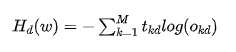
This is the loss function for a single sample d. For all samples, it can be expressed as:
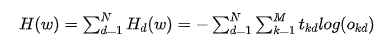
Where  represents the desired output of the k-th neuron in the output layer for sample d,
  represents the actual output of the k-th neuron in the output layer for sample d, and
  represents the logarithm of the output
  .
.
Xiao Ming looked at the formula and asked in confusion: “What is the specific physical meaning of the cross-entropy loss function?”
Dr. Ai asked Xiao Ming back: “Do you remember what the expected outputs look like when we used cat and dog recognition as an example?”
Xiao Ming thought for a moment and replied: “One output represents a cat, and the other represents a dog. When the input is a cat, the expected output for the cat is 1, and for the dog, it is 0. When the input is a dog, it is the opposite.”
Dr. Ai said: “Correct. The expected outputs of 1 or 0 can be regarded as probability values.”
Xiao Ming asked: “How do we obtain a probability at the output layer of the neural network?”
Dr. Ai said: “To obtain probability values at the output layer, we need to satisfy two main properties of probabilities: one is that the values lie between 0 and 1, and the other is that the sum of all outputs equals 1. To achieve this, we need to use an activation function called softmax. This activation function differs from the activation functions we discussed earlier, which only act on a single neuron; softmax acts on all neurons in the output layer.”
Let 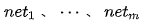 represent the outputs of each neuron in the output layer before applying the activation function. After applying the softmax activation function, the output of the i-th neuron
  is:
is:
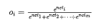
It is easy to verify that such output values can satisfy the two properties of probabilities. Thus, we can treat the outputs of the neural network as probabilities, and we will see that this usage is very common.
Dr. Ai continued explaining: “Returning to your question about the physical meaning of the cross-entropy loss function, from a probability perspective, we want the output probability corresponding to the input to be large, while the probabilities for other outputs should be small. For a classification problem, when the input sample is given, only one of the M expected outputs is 1, while the others are 0. Therefore, in the cross-entropy calculation, the summation part actually has only one non-zero term, while the others are zero, so:
We minimize  . Ignoring the negative sign, we are actually maximizing
  , which is to maximize the probability value corresponding to sample d’s output. Since the output layer uses the softmax activation function, as the output corresponding to sample d increases, the outputs of the other neurons must naturally decrease.
Xiao Ming: “So that’s the meaning! I understand now. What are the uses of the sum of squared errors loss function and the cross-entropy loss function?”
Dr. Ai: “Xiao Ming, you asked a very good question. From the analysis above, the cross-entropy loss function is more suitable for classification problems, directly optimizing the output probability values, while the sum of squared errors loss function is more suitable for prediction problems.”
Xiao Ming, not understanding what a prediction problem was, immediately asked: “Dr. Ai, what is a prediction problem?”
Dr. Ai gave an example: “If the output is to predict a specific numerical value, that is a prediction problem. For instance, predicting tomorrow’s highest temperature based on today’s weather conditions is a prediction problem because we are predicting a specific value for temperature.”
After Dr. Ai’s careful explanation, Xiao Ming finally understood what a neural network is and how neural networks are trained. After bidding farewell to Dr. Ai, he returned home with a wealth of knowledge.
Xiao Ming’s Study Notes
Neural networks are trained by optimizing the minimization of loss functions, which include the sum of squared errors and cross-entropy loss functions. Different loss functions are applied in different scenarios; the sum of squared errors loss function is generally used for solving prediction problems, while the cross-entropy loss function is generally used for solving classification problems.
The BP algorithm is a commonly used optimization method for neural networks, derived from the gradient descent algorithm. Its characteristic is that it provides a method for calculating errors through backpropagation, starting from the output layer and computing errors layer by layer to achieve weight updates.
The BP algorithm that uses only one sample at a time is called stochastic gradient descent, while the BP algorithm that uses several samples at a time is called batch gradient descent. The batch gradient descent algorithm is the most commonly used optimization algorithm for neural networks.
The BP algorithm is an iterative process that repeatedly uses samples from the training set to train the neural network. The use of all samples in the training set once is called one epoch, and generally, multiple epochs are needed to complete the training of the neural network.
Long press the QR code to follow CAAI for more media matrices

Official WeChat

Member Number

English Official WeChat
Click “Read the original text” to view the correction list and obtain the PPT