Top 10 Deep Learning Algorithms

Since the concept of deep learning was proposed in 2006, almost 20 years have passed. As a revolution in the field of artificial intelligence, deep learning has given rise to many influential algorithms. So, what do you think are the top 10 deep learning algorithms?

Here are my top 10 deep learning algorithms, which hold significant positions in terms of innovation, application value, and influence.

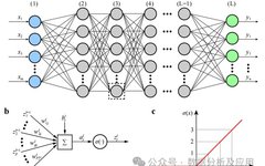
Background: Deep Neural Networks (DNN), also known as Multi-Layer Perceptrons, are the most common deep learning algorithms. Initially, they were questioned due to computational bottlenecks, but breakthroughs were only achieved in recent years with the explosion of computing power and data.

Model Principle: It is a neural network that contains multiple hidden layers. Each layer passes its input to the next layer and uses non-linear activation functions to introduce non-linear characteristics of learning. By combining these non-linear transformations, DNN can learn complex feature representations of input data.

Model Training: The weights are updated using the backpropagation algorithm and gradient descent optimization. During training, the gradient of the loss function with respect to the weights is calculated, and then gradient descent or other optimization algorithms are used to update the weights to minimize the loss function.

Advantages: It can learn complex features of input data and capture non-linear relationships. It has strong feature learning and representation capabilities.

Disadvantages: As the depth of the network increases, the vanishing gradient problem becomes severe, leading to unstable training. It is prone to local minima and may require complex initialization strategies and regularization techniques.

Use Cases: Image classification, speech recognition, natural language processing, recommendation systems, etc.

Python Example Code:

import numpy as np
from keras.models import Sequential
from keras.layers import Dense
# Assume there are 10 input features and 3 output classes  
input_dim = 10
num_classes = 3
# Create DNN model  
model = Sequential()
model.add(Dense(64, activation='relu', input_shape=(input_dim,)))
model.add(Dense(32, activation='relu'))
model.add(Dense(num_classes, activation='softmax'))
# Compile model, choose optimizer and loss function  
model.compile(optimizer='adam', loss='categorical_crossentropy', metrics=['accuracy'])
# Assume there are 100 samples of training data and labels  
X_train = np.random.rand(100, input_dim)
y_train = np.random.randint(0, 2, size=(100, num_classes))
# Train model  
model.fit(X_train, y_train, epochs=10)

2. Convolutional Neural Networks (CNN)

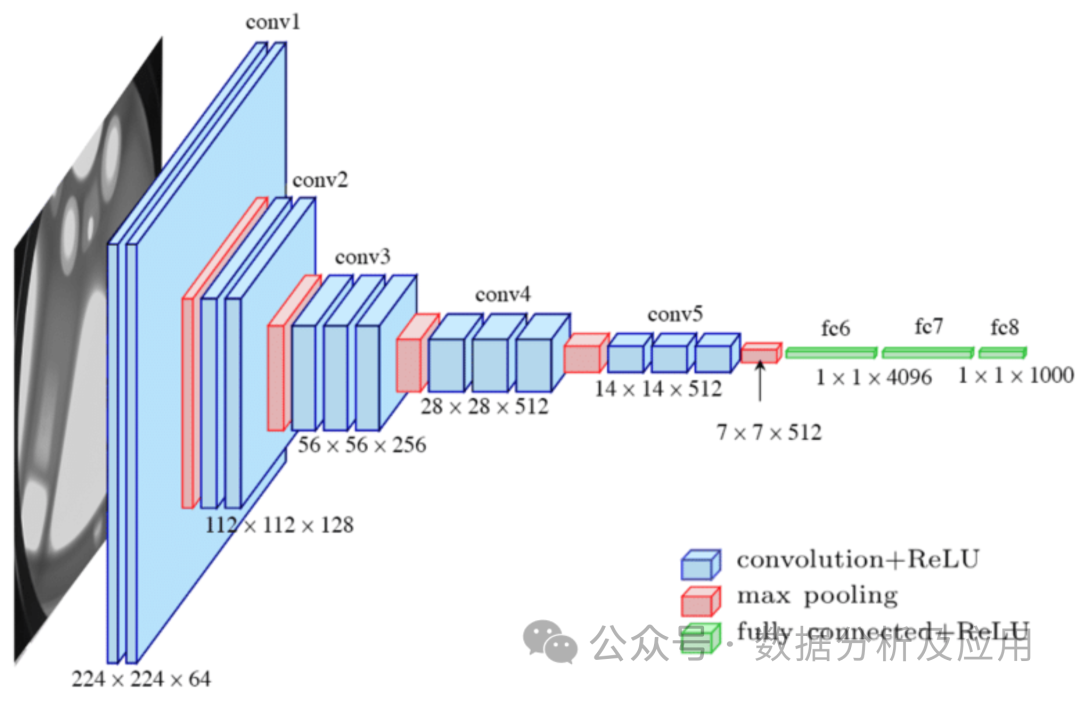
Model Principle: Convolutional Neural Networks (CNN) are designed specifically for processing image data, with LeNet designed by LeCun being the pioneering work of CNN. CNN captures local features using convolutional layers and reduces data dimensions through pooling layers. The convolutional layer performs local convolution operations on the input data and uses a parameter sharing mechanism to reduce the number of parameters in the model. The pooling layer downsamples the output from the convolutional layer to reduce data dimensions and computational complexity. This structure is particularly well-suited for processing image data.

Model Training: We use backpropagation and gradient descent optimization algorithms to update the weights. During training, we calculate the gradient of the loss function with respect to the weights and then update the weights using gradient descent or other optimization algorithms to minimize the loss function.

Advantages: It can effectively handle image data and capture local features. It has fewer parameters, reducing the risk of overfitting.

Disadvantages: It may not be suitable for sequential data or long-distance dependencies. It may require complex preprocessing of input data.

Use Cases: Image classification, object detection, semantic segmentation, etc.

Python Example Code:

from keras.models import Sequential
from keras.layers import Conv2D, MaxPooling2D, Flatten, Dense
# Assume the input image shape is 64x64 pixels with 3 color channels  
input_shape = (64, 64, 3)
# Create CNN model  
model = Sequential()
model.add(Conv2D(32, (3, 3), activation='relu', input_shape=input_shape))
model.add(MaxPooling2D((2, 2)))
model.add(Conv2D(64, (3, 3), activation='relu'))
model.add(Flatten())
model.add(Dense(128, activation='relu'))
model.add(Dense(num_classes, activation='softmax'))
# Compile model, choose optimizer and loss function  
model.compile(optimizer='adam', loss='categorical_crossentropy', metrics=['accuracy'])
# Assume there are 100 samples of training data and labels  
X_train = np.random.rand(100, *input_shape)
y_train = np.random.randint(0, 2, size=(100, num_classes))
# Train model  
model.fit(X_train, y_train, epochs=10)

3. Residual Networks (ResNet)

With the rapid development of deep learning, deep neural networks have achieved significant success in various fields. However, the training of deep neural networks faces issues such as vanishing gradients and model degradation, which limit the depth and performance of the network. To address these issues, Residual Networks (ResNet) were proposed.

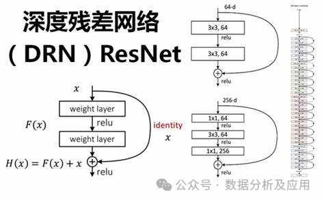
Model Principle: ResNet addresses the vanishing gradient and model degradation issues in deep neural networks by introducing “residual blocks.” A residual block consists of a “skip connection” and one or more non-linear layers, allowing gradients to be directly backpropagated from later layers to earlier layers, thus better training deep neural networks. In this way, ResNet can construct very deep network structures and achieve excellent performance across multiple tasks.

Model Training: Training ResNet typically uses backpropagation and optimization algorithms (such as stochastic gradient descent). During training, the gradient of the loss function with respect to the weights is calculated, and optimization algorithms are used to update the weights to minimize the loss function. Additionally, techniques such as regularization and ensemble learning can be adopted to accelerate the training process and improve the model’s generalization ability.

Advantages:

1. Addresses vanishing gradient and model degradation issues: By introducing residual blocks and skip connections, ResNet can better train deep neural networks and avoid vanishing gradient and model degradation issues.

2. Constructs very deep network structures: By addressing vanishing gradients and model degradation issues, ResNet can construct very deep network structures, thereby improving model performance.

3. Achieves excellent performance across multiple tasks: Due to its strong feature learning and representation capabilities, ResNet has achieved excellent performance in various tasks such as image classification and object detection.

Disadvantages:

1. High computational cost: Since ResNet typically constructs very deep network structures, it requires significant computational resources and time for training.

2. Difficult parameter tuning: ResNet has numerous parameters, requiring substantial time and effort for tuning and hyperparameter selection.

3. Sensitive to initialization weights: ResNet is sensitive to the choice of initialization weights; inappropriate initialization may lead to unstable training or overfitting issues.

Use Cases: ResNet has a wide range of applications in computer vision, such as image classification, object detection, and face recognition. Additionally, ResNet can also be used in natural language processing and speech recognition.

Python Example Code (Simplified): In this simplified example, we will demonstrate how to build a simple ResNet model using the Keras library.

from keras.models import Sequential
from keras.layers import Conv2D, Add, Activation, BatchNormalization, Shortcut
def residual_block(input, filters):
    x = Conv2D(filters=filters, kernel_size=(3, 3), padding='same')(input)
    x = BatchNormalization()(x)
    x = Activation('relu')(x)
    x = Conv2D(filters=filters, kernel_size=(3, 3), padding='same')(x)
    x = BatchNormalization()(x)
    x = Activation('relu')(x)
    return x

4. LSTM (Long Short-Term Memory Networks)

When dealing with sequential data, traditional Recurrent Neural Networks (RNNs) face issues such as vanishing gradients and model degradation, which limit the depth and performance of the network. To address these issues, LSTMs were proposed.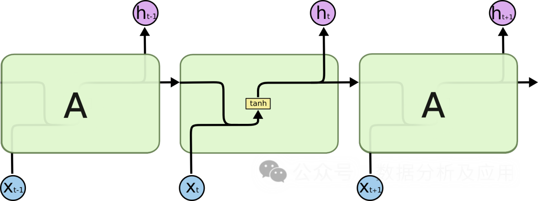

Model Principle: LSTMs introduce “gating” mechanisms to control the flow of information, thus solving the vanishing gradient and model degradation issues. LSTMs have three gating mechanisms: input gate, forget gate, and output gate. The input gate determines the entry of new information, the forget gate determines the forgetting of old information, and the output gate determines the final output information. Through these gating mechanisms, LSTMs can perform better on long-term dependency issues.

Model Training: LSTM training typically uses backpropagation and optimization algorithms (such as stochastic gradient descent). During training, the gradient of the loss function with respect to the weights is calculated, and optimization algorithms are used to update the weights to minimize the loss function. Additionally, techniques such as regularization and ensemble learning can be adopted to accelerate the training process and improve the model’s generalization ability.

Advantages:

1. Addresses vanishing gradient and model degradation issues: By introducing gating mechanisms, LSTMs can better handle long-term dependency issues, avoiding vanishing gradients and model degradation.

2. Constructs very deep network structures: By addressing vanishing gradients and model degradation issues, LSTMs can construct very deep network structures, thereby improving model performance.

3. Achieves excellent performance across multiple tasks: Due to their strong feature learning and representation capabilities, LSTMs have achieved excellent performance in various tasks such as text generation, speech recognition, and machine translation.

Disadvantages:

1. Difficult parameter tuning: LSTMs have numerous parameters, requiring substantial time and effort for tuning and hyperparameter selection.

2. Sensitive to initialization weights: LSTMs are sensitive to the choice of initialization weights; inappropriate initialization may lead to unstable training or overfitting issues.

3. High computational cost: Since LSTMs typically construct very deep network structures, they require significant computational resources and time for training.

Use Cases: LSTMs have a wide range of applications in natural language processing, such as text generation, machine translation, and speech recognition. Additionally, LSTMs can also be used in time series analysis and recommendation systems.

Python Example Code (Simplified):

from keras.models import Sequential
from keras.layers import LSTM, Dense
def lstm_model(input_shape, num_classes):
    model = Sequential()
    model.add(LSTM(units=128, input_shape=input_shape))  # Add an LSTM layer  
    model.add(Dense(units=num_classes, activation='softmax'))  # Add a fully connected layer  
    return model

5. Word2Vec

The Word2Vec model is a pioneering work in representation learning. It is a (shallow) neural network model developed by Google’s scientists for natural language processing. The goal of the Word2Vec model is to vectorize each word into a fixed-size vector so that similar words can be mapped to nearby vector spaces.

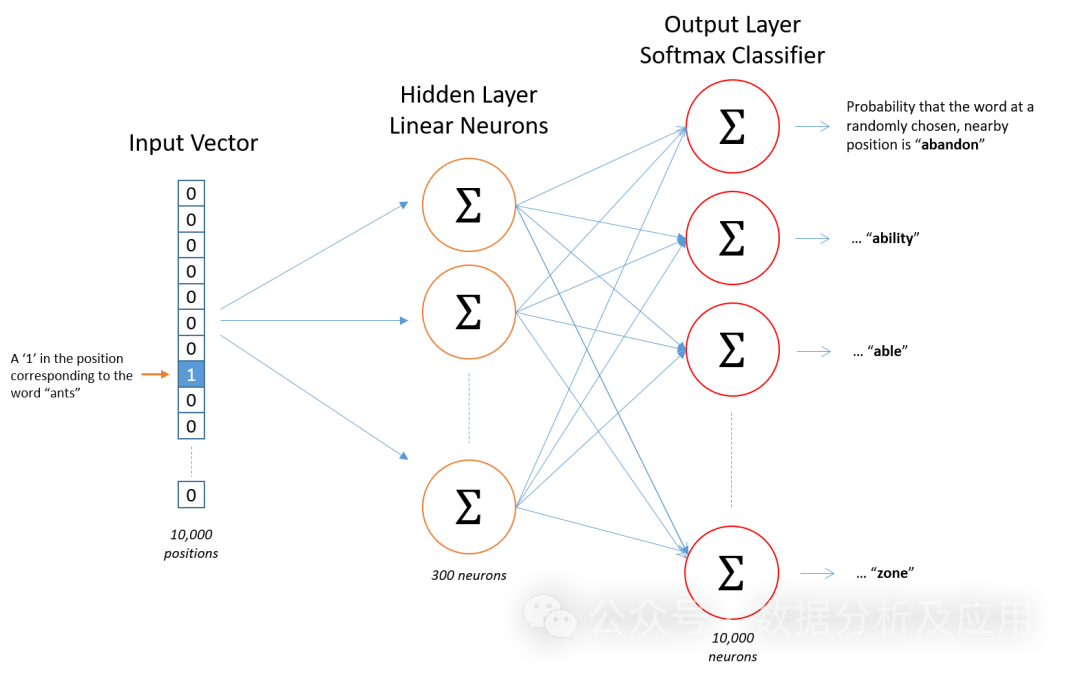
Model Principle

The Word2Vec model is based on neural networks, utilizing input words to predict their context words. During training, the model attempts to learn the vector representation of each word so that the words appearing in a given context are as close as possible to the target word’s vector representation. This training method is called “Skip-gram” or “Continuous Bag of Words” (CBOW).

Model Training

Training the Word2Vec model requires a large amount of text data. First, the text data is preprocessed into a series of words or n-grams. Then, a neural network is used to train the context of these words or n-grams. During training, the model continuously adjusts the vector representation of words to minimize prediction errors.

Advantages

1. Semantic Similarity: Word2Vec can learn the semantic relationships between words, where similar words are close together in vector space.

2. Efficient Training: The training process of Word2Vec is relatively efficient and can be trained on large-scale text data.

3. Interpretability: The word vectors of Word2Vec have a certain degree of interpretability and can be used for tasks such as clustering, classification, and semantic similarity calculations.

Disadvantages

1. Sparsity of Data: For many words not appearing in the training data, Word2Vec may not be able to generate accurate vector representations.

2. Context Window: Word2Vec only considers a fixed-size context, which may overlook more distant dependencies.

3. Computational Complexity: The training and inference processes of Word2Vec require significant computational resources.

4. Parameter Tuning: The performance of Word2Vec heavily depends on the settings of hyperparameters (such as vector dimensions, window size, learning rate, etc.).

Use Cases

Word2Vec is widely used in various natural language processing tasks, such as text classification, sentiment analysis, information extraction, etc. For example, Word2Vec can be used to identify the sentiment tendency (positive or negative) of news reports or extract key entities or concepts from large amounts of text.

Python Example Code

from gensim.models import Word2Vec  
from nltk.tokenize import word_tokenize  
from nltk.corpus import abc  
import nltk    
# Download and load the abc corpus  
nltk.download('abc')  
corpus = abc.sents()    
# Tokenize the corpus and convert to lowercase  
sentences = [[word.lower() for word in word_tokenize(text)] for text in corpus]    
# Train the Word2Vec model  
model = Word2Vec(sentences, vector_size=100, window=5, min_count=5, workers=4)    
# Find the vector representation of the word "the"  
vector = model.wv['the']    
# Calculate similarity with other words  
similarity = model.wv.similarity('the', 'of')    
# Print similarity value  
print(similarity)

6. Transformer

Background: In the early stages of deep learning, Convolutional Neural Networks (CNNs) achieved significant success in image recognition and natural language processing. However, as task complexity increased, sequence-to-sequence (Seq2Seq) models and Recurrent Neural Networks (RNNs) became commonly used methods for processing sequential data. Although RNNs and their variants perform well on certain tasks, they tend to encounter vanishing gradient and model degradation issues when processing long sequences. To address these issues, the Transformer model was proposed. Subsequent large models such as GPT and BERT have achieved outstanding performance based on the Transformer!

Model Principle: The Transformer model consists mainly of two parts: the encoder and the decoder. Each part consists of multiple identical “layers.” Each layer contains two sub-layers: a self-attention sub-layer and a linear feedforward neural network sub-layer. The self-attention sub-layer computes the representation of each position in the input sequence using a dot-product attention mechanism, while the linear feedforward neural network sub-layer takes the output of the self-attention layer as input and produces an output representation. Additionally, both the encoder and decoder contain a positional encoding layer to capture positional information in the input sequence.

Model Training: Training the Transformer model typically uses backpropagation and optimization algorithms (such as stochastic gradient descent). During training, the gradient of the loss function with respect to the weights is calculated, and optimization algorithms are used to update the weights to minimize the loss function. Additionally, techniques such as regularization and ensemble learning can be adopted to accelerate the training process and improve the model’s generalization ability.

Advantages:

1. Addresses vanishing gradient and model degradation issues: The Transformer model uses a self-attention mechanism to better capture long-term dependencies in sequences, thus avoiding the vanishing gradient and model degradation issues.

2. Efficient parallel computing capability: Since the computations in the Transformer model can be parallelized, training and inference can be done quickly on GPUs.

3. Achieves excellent performance across multiple tasks: Due to its strong feature learning and representation capabilities, the Transformer model has achieved excellent performance in various tasks such as machine translation, text classification, and speech recognition.

Disadvantages:

1. High computational cost: Since the computations in the Transformer model can be parallelized, it requires significant computational resources for training and inference.

2. Sensitive to initialization weights: The Transformer model is sensitive to the choice of initialization weights; inappropriate initialization may lead to unstable training or overfitting issues.

3. Inability to learn long-term dependencies: Although the Transformer model addresses vanishing gradients and model degradation issues, challenges remain when processing very long sequences.

Use Cases: The Transformer model has a wide range of applications in natural language processing, such as machine translation, text classification, and text generation. Additionally, the Transformer model can also be used in image recognition and speech recognition.

Python Example Code (Simplified):

import torch  
import torch.nn as nn  
import torch.nn.functional as F  

class TransformerModel(nn.Module):  
    def __init__(self, vocab_size, embedding_dim, num_heads, num_layers, dropout_rate=0.5):  
        super(TransformerModel, self).__init__()  
        self.embedding = nn.Embedding(vocab_size, embedding_dim)  
        self.transformer = nn.Transformer(d_model=embedding_dim, nhead=num_heads, num_encoder_layers=num_layers, num_decoder_layers=num_layers, dropout=dropout_rate)  
        self.fc = nn.Linear(embedding_dim, vocab_size)  
      
    def forward(self, src, tgt):  
        embedded = self.embedding(src)  
        output = self.transformer(embedded)  
        output = self.fc(output)  
        return output
pip install transformers

7. Generative Adversarial Networks (GAN)

The idea of GAN comes from zero-sum games in game theory, where one player tries to generate the most realistic fake data while the other player attempts to distinguish between real data and fake data. GAN evolved from the Monty Hall problem (a problem combining generative and discriminative models), but unlike the Monty Hall problem, GAN does not emphasize approximating certain probability distributions or generating specific samples; instead, it directly uses generative and discriminative models in opposition.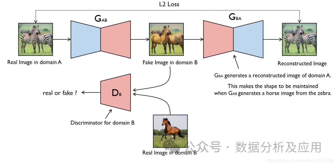

Model Principle: GAN consists of two parts: the generator and the discriminator. The generator’s task is to generate fake data, while the discriminator’s task is to determine whether the input data comes from the real dataset or is generated by the generator. During training, the generator and discriminator engage in opposition, continually adjusting parameters until a balance is reached. At this point, the fake data generated by the generator is realistic enough that the discriminator cannot distinguish between real and fake data.

Model Training: The training process of GAN is an optimization problem. In each training step, the generator generates fake data using the current parameters, and then the discriminator assesses whether this data is real or generated. Based on this assessment, the parameters of the discriminator are updated. Simultaneously, to prevent overfitting of the discriminator, the generator must also be trained to produce fake data that can deceive the discriminator. This process is repeated until a balance is achieved.

Advantages:

1. Strong generative capabilities: GAN can learn the intrinsic structure and distribution of data, thereby generating very realistic fake data.

2. No explicit supervision required: The training process of GAN does not require explicit label information; only real data is needed.

3. High flexibility: GAN can be combined with other models, such as forming AutoGAN with autoencoders or forming DCGAN with convolutional neural networks.

Disadvantages:

1. Unstable training: The training process of GAN is unstable and prone to mode collapse, where the generator only produces one type of sample, making it difficult for the discriminator to make accurate judgments.

2. Difficult debugging: Debugging GANs is challenging due to the complex interactions between the generator and discriminator.

3. Difficult to evaluate: Due to the strong generative capabilities of GANs, it is difficult to assess the authenticity and diversity of the generated fake data.

Use Cases:

1. Image generation: GANs are most commonly used for image generation tasks, capable of generating images in various styles, such as generating images based on text descriptions or transforming one image into another style.

2. Data augmentation: GANs can be used to generate fake data similar to real data to expand datasets or improve model generalization.

3. Image restoration: GANs can be used to repair defects in images or remove noise from images.

4. Video generation: Video generation based on GANs is currently a hot research topic, capable of generating videos in various styles.

Simple Python Example Code:

Below is a simple GAN example code implemented using PyTorch:

import torch
import torch.nn as nn
import torch.optim as optim
import torch.nn.functional as F
# Define the generator and discriminator network structures  
class Generator(nn.Module):
    def __init__(self, input_dim, output_dim):
        super(Generator, self).__init__()
        self.model = nn.Sequential(
            nn.Linear(input_dim, 128),
            nn.ReLU(),
            nn.Linear(128, output_dim),
            nn.Sigmoid()
        )
    def forward(self, x):
        return self.model(x)
class Discriminator(nn.Module):
    def __init__(self, input_dim):
        super(Discriminator, self).__init__()
        self.model = nn.Sequential(
            nn.Linear(input_dim, 128),
            nn.ReLU(),
            nn.Linear(128, 1),
            nn.Sigmoid()
        )
    def forward(self, x):
        return self.model(x)
# Instantiate generator and discriminator objects  
input_dim = 100  # Input dimension can be adjusted as needed  
output_dim = 784  # For the MNIST dataset, output dimension is 28*28=784  
gen = Generator(input_dim, output_dim)
disc = Discriminator(output_dim)
# Define loss function and optimizer  
criterion = nn.BCELoss()  # Binary cross-entropy loss suitable for the discriminator part of GAN and the generator's logistic loss part. However, it is more common to use the binary cross-entropy loss function (binary cross-entropy loss function).

8. Diffusion Models

The Diffusion model is a deep learning-based generative model primarily used for generating continuous data, such as images and audio. The core idea of the Diffusion model is to convert complex data distributions into simple Gaussian distributions by gradually adding noise and then generating data from the simple distribution by gradually removing noise.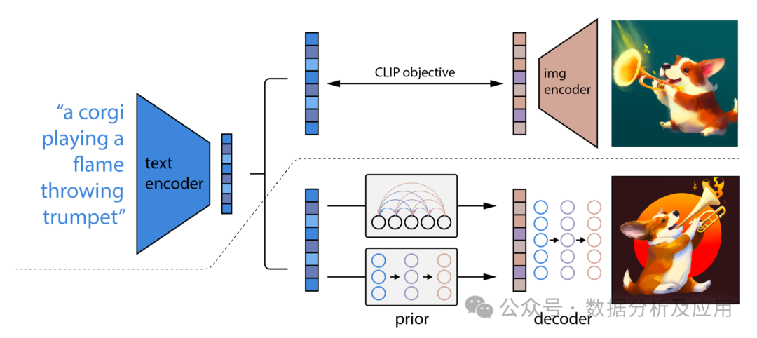

Model Principle
The Diffusion model consists of two main processes: the forward diffusion process and the reverse diffusion process.
Forward diffusion process:
Sample a data point (x_0) from the true data distribution.
In (T) time steps, gradually add noise to (x_0) to generate a series of noise data points (x_1, x_2, ..., x_T) that gradually deviate from the true data distribution.
This process can be viewed as gradually transforming the data distribution into a Gaussian distribution.
Reverse diffusion process (also known as the denoising process):
Starting from the noise data distribution (x_T), gradually remove noise to generate a series of data points (x_{T-1}, x_{T-2}, ..., x_0) that gradually approach the true data distribution.
This process is learned by a neural network to predict the noise at each step and uses this prediction to gradually denoise.
Model Training
Training the Diffusion model typically involves the following steps:
Forward diffusion: For each sample (x_0) in the training dataset, generate the corresponding noise sequence (x_1, x_2, ..., x_T) according to a predetermined noise scheduling scheme.
Noise prediction: For each time step (t), train a neural network to predict the noise in (x_t). This neural network is typically a Conditional Variational Autoencoder (CVAE), which takes (x_t) and time step (t) as inputs and outputs the predicted noise.
Optimization: Optimize the neural network parameters by minimizing the difference between the true noise and the predicted noise. The commonly used loss function is Mean Squared Error (MSE).
Advantages
Strong generative capabilities: The Diffusion model can generate high-quality and diverse data samples.
Progressive generation: The model can provide intermediate results during the generation process, which helps to understand the model's generation process.
Stable training: Compared to other generative models (such as GANs), the Diffusion model is generally easier to train and less prone to mode collapse issues.
Disadvantages
High computational cost: Due to the need for forward and reverse diffusion across multiple time steps, the training and generation processes of the Diffusion model are typically time-consuming.
High number of parameters: For each time step, a separate neural network is required for noise prediction, resulting in a large number of model parameters.
Use Cases
The Diffusion model is suitable for scenarios requiring continuous data generation, such as image generation, audio generation, and video generation. Additionally, due to the model's progressive generation characteristics, it can also be used for data interpolation and style transfer tasks.
Python Example Code
Below is a simplified example code for training a Diffusion model using the PyTorch library:
import torch  
import torch.nn as nn  
import torch.optim as optim    
# Assume we have a simple Diffusion model  
class DiffusionModel(nn.Module):      
    def __init__(self, input_dim, hidden_dim, num_timesteps):          
        super(DiffusionModel, self).__init__()          
        self.num_timesteps = num_timesteps          
        self.noises = nn.ModuleList([
            nn.Linear(input_dim, hidden_dim),
            nn.ReLU(),
            nn.Linear(hidden_dim, input_dim)
        ] for _ in range(num_timesteps))        
    def forward(self, x, t):          
        noise_prediction = self.noises[t](x)          
        return noise_prediction    
# Set model parameters  
input_dim = 784  # Assume input is a 28x28 grayscale image  
hidden_dim = 128  
num_timesteps = 1000    
# Initialize model  
model = DiffusionModel(input_dim, hidden_dim, num_timesteps)    
# Define loss function and optimizer  
criterion = nn.MSELoss()  
optimizer = optim.Adam(model.parameters(), lr=1e-3)

9. Graph Neural Networks (GNN)

Graph Neural Networks (GNN) are deep learning models specifically designed to handle graph-structured data. Many complex systems in the real world can be represented as graphs, such as social networks, molecular structures, and transportation networks. Traditional machine learning models face many challenges when dealing with these graph-structured data, while GNNs provide new solutions to these problems.
Model Principle:
The core idea of GNN is to learn feature representations of nodes in the graph through a neural network while considering the relationships between nodes. Specifically, GNN iteratively updates the representation of nodes by passing information from their neighbors, allowing similar communities or adjacent nodes to have similar representations. In each layer, nodes update their representations based on information from their neighbor nodes, thereby capturing complex patterns within the graph.
Model Training:
Training GNNs typically employs gradient-based optimization algorithms like stochastic gradient descent (SGD). During training, the gradient of the loss function is calculated using backpropagation, and the weights of the neural network are updated. Common loss functions include cross-entropy loss for node classification and binary cross-entropy loss for link prediction.
Advantages:
Strong representation capabilities: GNNs can effectively capture complex patterns in graph structures, achieving good results in tasks like node classification and link prediction.
Natural handling of graph-structured data: GNNs process graph-structured data directly without needing to convert the graph into matrix form, avoiding the computational and storage overhead of large sparse matrices.
Strong scalability: GNNs can stack more layers to capture more complex patterns, offering strong scalability.
Disadvantages:
High computational complexity: As the number of nodes and edges in the graph increases, the computational complexity of GNNs also rises sharply, potentially leading to longer training times.
Difficult parameter tuning: GNNs have many hyperparameters, such as neighborhood size, number of layers, learning rate, etc. Tuning these parameters may require in-depth understanding of the task.
Different adaptability for undirected and directed graphs: GNNs were initially designed for undirected graphs, and their adaptability for directed graphs may be poorer.
Use Cases:
Social network analysis: In social networks, relationships between users can be represented as graphs. GNNs can analyze user similarities, community discovery, influence propagation, and more.
Molecular structure prediction: In the field of chemistry, molecular structures can be represented as graphs. Training GNNs can predict the properties of molecules and chemical reactions.
Recommendation systems: Recommendation systems can utilize user behavior data to build graphs, then use GNNs to capture user behavior patterns for precise recommendations.
Knowledge graphs: Knowledge graphs can be seen as a special type of graph-structured data. GNNs can conduct in-depth analysis of entities and relationships within knowledge graphs.
Simple Python Example Code:
import torch from torch_geometric.datasets import Planetoid from torch_geometric.nn import GCNConv from torch_geometric.data import DataLoader import time # Load the Cora dataset dataset = Planetoid(root=’/tmp/Cora’, name=’Cora’) # Define the GNN model class GNN(torch.nn.Module):def __init__(self, in_channels, hidden_channels, out_channels): super(GNN, self).__init__() self.conv1 = GCNConv(in_channels, hidden_channels) self.conv2 = GCNConv(hidden_channels, out_channels) def forward(self, data): x, edge_index = data.x, data.edge_index x = self.conv1(x, edge_index) x = F.relu(x) x = F.dropout(x, training=self.training) x = self.conv2(x, edge_index) return F.log_softmax(x, dim=1) # Define hyperparameters and model training process num_epochs = 1000lr = 0.01hidden_channels = 16out_channels = dataset.num_classes data = dataset[0] # Use the first data in the dataset as example data model = GNN(dataset.num_features, hidden_channels, out_channels) optimizer = torch.optim.Adam(model.parameters(), lr=lr) data = DataLoader([data], batch_size=1) # Convert dataset to DataLoader object for batch training and evaluation model.train() # Set model to training mode for epoch in range(num_epochs): for data in data: # In each epoch, iterate through the entire dataset once optimizer.zero_grad() # Clear gradients out = model(data) # Forward pass, calculate output and loss function value loss = F.nll_loss(out[data.train_mask], data.y[data.train_mask]) # Calculate loss function value, using negative log likelihood loss function as example loss function loss.backward() # Backpropagation, calculate gradients optimizer.step() # Update weight parameters

10. Deep Q-Networks (DQN)

In traditional reinforcement learning algorithms, agents use a Q-table to store estimates of state-action value functions. However, this method encounters limitations when dealing with high-dimensional state and action spaces. To address this issue, DQN is a deep reinforcement learning algorithm that introduces deep learning techniques to approximate the state-action value function, enabling it to handle more complex problems.
Model Principle:
DQN uses a neural network (called a deep Q network) to approximate the state-action value function. This neural network takes the current state as input and outputs the Q-values for each action. During training, the agent updates the neural network weights by continuously interacting with the environment to gradually approximate the optimal Q-value function.
Model Training:
The training process of DQN includes two phases: the offline phase and the online phase. In the offline phase, the agent randomly samples a batch of experiences (i.e., state, action, reward, and next state) from the experience replay buffer and uses these experiences to update the deep Q network. In the online phase, the agent selects and executes the best action using the current state and deep Q network, storing new experiences in the experience replay buffer.
Advantages:
Handles high-dimensional state and action spaces: DQN can address complex problems with high-dimensional state and action spaces, making it widely applicable in many fields.
Reduces data dependency: By using the experience replay buffer, DQN can train effectively with limited samples.
Flexibility: DQN can be combined with other reinforcement learning algorithms and techniques to further enhance performance and expand its application scope.
Disadvantages:
Unstable training: In some cases, DQN training may be unstable, leading to learning failures or performance declines.
Exploration strategy: DQN requires an effective exploration strategy to explore the environment and collect sufficient experiences. Choosing the right exploration strategy is crucial as it can affect learning speed and final performance.
Need for target networks: To stabilize training, DQN often requires the use of target networks to update the Q-value function. This increases the complexity of the algorithm and requires additional parameter tuning.
Use Cases:
DQN has been widely applied in various game AI tasks, such as Go, card games, and more. Additionally, it has been applied in other fields such as robotic control, natural language processing, and autonomous driving.
Python Example Code:
import numpy as np import tensorflow as tf from tensorflow.keras.models import Sequential from tensorflow.keras.layers import Dense, Dropout class DQN: def __init__(self, state_size, action_size): self.state_size = state_size self.action_size = action_size self.memory = np.zeros((MEM_CAPACITY, state_size * 2 + 2)) self.gamma = 0.95self.epsilon = 1.0self.epsilon_min = 0.01self.epsilon_decay = 0.995self.learning_rate = 0.005self.model = self.create_model() def create_model(self): model = Sequential() model.add(Dense(24, input_dim=self.state_size, activation=’relu’)) model.add(Dense(24, activation=’relu’)) model.add(Dense(self.action_size, activation=’linear’)) model.compile(loss=’mse’, optimizer=tf.keras.optimizers.Adam(lr=self.learning_rate)) return model def remember(self, state, action, reward, next_state, done): self.memory[self.memory_counter % MEM_CAPACITY, :] = [state, action, reward, next_state, done] self.memory_counter += 1def act(self, state): if np.random.rand() <= self.epsilon:return np.random.randint(self.action_size) act_values = self.model.predict(state) return np.argmax(act_values[0]) def replay(self): batch_size = 32 start = np.random.randint(0, self.memory_counter – batch_size, batch_size) sample = self.memory[start:start + batch_size] states = np.array([s[0] for s in sample]) actions = np.array([s[1] for s in sample]) rewards = np.array([s[2] for s in sample]) next_states = np.array([s[3] for s in sample]) done = np.array([s[4] for s in sample]) target = self.model.predict(next_states) target_q = rewards + (1 – done) * self.gamma * np.max(target, axis=1) target_q = np.asarray([target_q[i] for i in range(batch_size)]) target = self.model.predict(states) indices = np.arange(batch_size) for i in range(batch_size): if done[i]: continue # no GAE calc for terminal states (if you want to include terminal states see line 84) target[indices[i]] = rewards[i] + self.gamma * target_q[indices[i]] # GAE formula line 84 (https://arxiv.org/pdf/1506.02438v5) instead of line 85 (https://arxiv.org/pdf/1506.02438v5) (if you want to include terminal states see line 84) indices[i] += batch_size # resets the indices for the next iteration (https://github.com/ikostrikov/pytorch-a2c-ppo-acktr-gail/blob/master/a2c.py#L173) (if you want to include terminal states see line 84) target[indices[i]] = target[indices[i]] # resets the indices for the next iteration (https://github.com/ikostrikov/pytorch-a2c-ppo-acktr-gail/blob/master/a2c.py#L173) (if you want to include terminal states see line 84) (https://github.com/ikostrikov/pytorch-a2c-ppo-acktr-gail/blob/master/a2c.py#L173)