Selected from efficientdl.com
Author: LORENZ KUHN
Translated by: Machine Heart
Editor: Chen Ping
Master these 17 methods to accelerate your PyTorch deep learning training with minimal effort.
Recently, a post on Reddit gained immense popularity. The topic was about how to speed up PyTorch training. The original author is LORENZ KUHN, a master’s student in computer science from ETH Zurich, who introduces us to the 17 most efficient and effortless methods to train deep models using PyTorch.

All methods mentioned assume that you are training the model in a GPU environment. The specific content is as follows.
17 Methods to Accelerate PyTorch Training
1. Consider Changing the Learning Rate Schedule
The choice of learning rate schedule greatly affects the convergence speed and generalization ability of the model. Leslie N. Smith et al. proposed cyclical learning rates and the 1Cycle learning rate schedule in the papers “Cyclical Learning Rates for Training Neural Networks” and “Super-Convergence: Very Fast Training of Neural Networks Using Large Learning Rates”. Later, Jeremy Howard and Sylvain Gugger from fast.ai promoted it. The following figure illustrates the 1Cycle learning rate schedule:
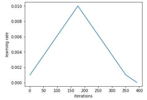
Sylvain wrote: 1Cycle includes two equal-length phases, one phase is from a lower learning rate to a higher learning rate, and the other returns to the lowest level. The maximum value comes from the value selected by the learning rate finder, and the smaller value can be ten times lower. The length of this cycle should be slightly less than the total number of epochs, and in the final stages of training, we should allow the learning rate to be several orders of magnitude lower than the minimum.
Compared to traditional learning rate schedules, this schedule achieves significant speedup in the best case (which Smith calls super-convergence). For example, using the 1Cycle strategy to train ResNet-56 on the ImageNet dataset reduced the training iterations to 1/10 of the original, yet the model performance can still match that in the original paper. This schedule seems to perform well across common architectures and optimizers.
Pytorch has already implemented these two methods: “torch.optim.lr_scheduler.CyclicLR” and “torch.optim.lr_scheduler.OneCycleLR”.
Reference documentation: https://pytorch.org/docs/stable/optim.html
2. Use Multiple Workers and Pin Memory in DataLoader
When using torch.utils.data.DataLoader, set num_workers > 0 instead of the default 0, and set pin_memory=True instead of the default False.
The senior CUDA deep learning algorithm software engineer Szymon Micacz from NVIDIA achieved a 2x speedup in a single epoch using four workers and pinned memory. A rule of thumb for choosing the number of workers is to set it to four times the number of available GPUs; setting it higher or lower will reduce training speed. Note that increasing num_workers will increase CPU memory consumption.
Maximizing batch size is a somewhat controversial viewpoint. Generally, if you maximize batch size within the limits of GPU memory, your training speed will be faster. However, you must also adjust other hyperparameters, such as learning rate. A good rule of thumb is to double the learning rate when you double the batch size.
OpenAI’s paper “An Empirical Model of Large-Batch Training” demonstrates how many steps different batch sizes require to converge. In the article “How to get 4x speedup and better generalization using the right batch size”, author Daniel Huynh conducted experiments with different batch sizes (also using the 1Cycle strategy discussed above). Ultimately, he increased the batch size from 64 to 512, achieving a 4x speedup.
However, the downside of using a large batch is that it may lead to poorer generalization ability compared to using a small batch.
4. Use Automatic Mixed Precision (AMP)
PyTorch version 1.6 includes a native implementation for automatic mixed precision training. It is worth mentioning that certain operations run faster in half-precision (FP16) compared to single precision (FP32) without losing accuracy. AMP automatically decides which precision to use for which operations. This can accelerate training speed and reduce memory usage.
In the best case, AMP usage looks like this:
import torch# Creates once at the beginning of training
scaler = torch.cuda.amp.GradScaler()

for data, label in data_iter:
    optimizer.zero_grad()  # Casts operations to mixed precision
    with torch.cuda.amp.autocast():
        loss = model(data)
    # Scales the loss, and calls backward() to create scaled gradients
    scaler.scale(loss).backward()
    # Unscales gradients and calls or skips optimizer.step()
    scaler.step(optimizer)
    # Updates the scale for next iteration
    scaler.update()
5. Consider Using Another Optimizer
AdamW is an Adam variant with weight decay (instead of L2 regularization) promoted by fast.ai, implemented in PyTorch as torch.optim.AdamW. AdamW seems to consistently outperform Adam in both error and training time.
Both Adam and AdamW work well with the aforementioned 1Cycle strategy.
Currently, some non-native optimizers have also gained significant attention, most notably LARS and LAMB. NVIDIA’s APEX implements fused versions of some common optimizers like Adam. This implementation avoids multiple passes with GPU memory compared to the Adam implementation in PyTorch, improving speed by 5%.
If your model architecture and input size remain unchanged, set torch.backends.cudnn.benchmark = True.
7. Be Careful of Frequent Data Transfers Between CPU and GPU
Frequent use of tensor.cpu() to transfer tensors from GPU to CPU (or using tensor.cuda() to transfer tensors from CPU to GPU) is very costly. item() and .numpy() can also be used. Use .detach() instead.
If you create a new tensor, you can assign it to the GPU using the keyword argument device=torch.device(‘cuda:0’).
If you need to transfer data, you can use .to(non_blocking=True), as long as there are no synchronization points after the transfer.
8. Use Gradient/Activation Checkpointing
Checkpointing works by trading computation for memory, not storing all intermediate activations of the computation graph for the backward pass, but instead recalculating these activations. We can apply it to any part of the model.
Specifically, in the forward pass, the function runs with torch.no_grad() and does not store intermediate activations. Instead, it saves the input tuple and function parameters in the forward pass. In the backward pass, the input and function are retrieved, and the forward pass is computed again on the function. Then track the intermediate activations and use these activation values to compute gradients.
Thus, while this may slightly increase the runtime for a given batch size, it significantly reduces memory usage. This, in turn, will allow further increases in the batch size used, thereby improving GPU utilization.
Although checkpointing is implemented via torch.utils.checkpoint, it still requires some thought and effort to implement correctly. Priya Goyal wrote a great tutorial introducing the key aspects of checkpointing.
Priya Goyal’s tutorial link:
https://github.com/prigoyal/pytorch_memonger/blob/master/tutorial/Checkpointing_for_PyTorch_models.ipynb
9. Use Gradient Accumulation
Another way to increase batch size is to accumulate gradients over multiple .backward() passes before calling optimizer.step().
The article by Thomas Wolf from Hugging Face, “Training Neural Nets on Larger Batches: Practical Tips for 1-GPU, Multi-GPU & Distributed setups,” explains how to use gradient accumulation. Gradient accumulation can be achieved as follows:
model.zero_grad()                                   # Reset gradients tensors
for i, (inputs, labels) in enumerate(training_set):
    predictions = model(inputs)                     # Forward pass
    loss = loss_function(predictions, labels)       # Compute loss function
    loss = loss / accumulation_steps                # Normalize our loss (if averaged)
    loss.backward()                                 # Backward pass
    if (i+1) % accumulation_steps == 0:             # Wait for several backward steps
        optimizer.step()                            # Now we can do an optimizer step
        model.zero_grad()                           # Reset gradients tensors
        if (i+1) % evaluation_steps == 0:           # Evaluate the model when we...
            evaluate_model()                        # ...have no gradients accumulate
This method is primarily developed to circumvent GPU memory limitations.
10. Use Distributed Data Parallel for Multi-GPU Training
There are many ways to accelerate distributed training, but a simple method is to use torch.nn.DistributedDataParallel instead of torch.nn.DataParallel. This way, each GPU will be driven by a dedicated CPU core, avoiding the GIL issues of DataParallel.
Distributed training documentation link: https://pytorch.org/tutorials/beginner/dist_overview.html
11. Set Gradients to None Instead of 0
Set gradients with .zero_grad(set_to_none=True) instead of .zero_grad(). Doing this allows the memory allocator to handle gradients instead of setting them to 0. As the documentation states, setting gradients to None provides moderate speedup, but don’t expect miracles. Note that this also has downsides, and further details can be found in the documentation.
Documentation link: https://pytorch.org/docs/stable/optim.html
12. Use .as_tensor() Instead of .tensor()
torch.tensor() always copies data. If you want to convert a numpy array, use torch.as_tensor() or torch.from_numpy() to avoid copying data.
13. Enable Debugging Tools When Necessary
PyTorch provides many debugging tools, such as autograd.profiler, autograd.grad_check, and autograd.anomaly_detection. Make sure to enable the debugger only when you need to debug, and turn it off promptly when not needed, as the debugger can slow down your training speed.
14. Use Gradient Clipping
To avoid the problem of exploding gradients in RNNs, some experiments and theories have confirmed that gradient clipping (gradient = min(gradient, threshold)) can accelerate convergence. HuggingFace’s Transformer implementation is a very clear example of how to use gradient clipping. Other methods mentioned in this article, such as AMP, can also be used.
In PyTorch, it can be implemented using torch.nn.utils.clip_grad_norm_.
15. Disable Bias Before BatchNorm
Disable the bias layer before starting the BatchNormalization layer. For a 2-D convolution layer, you can set the bias keyword to False: torch.nn.Conv2d(…, bias=False, …).
16. Disable Gradient Calculation During Validation
During validation, disable gradient calculation by setting: torch.no_grad().
17. Use Input and Batch Normalization
Be sure to check if the input is normalized? Is batch normalization used?
Original link: https://efficientdl.com/faster-deep-learning-in-pytorch-a-guide/
Nature Paper Online Sharing | The World’s Fastest Photonic AI Convolution Accelerator
The world’s fastest photonic AI convolution accelerator has been published in Nature. This research showcases an “optical neuromorphic processor” that operates more than 1000 times faster than any previous processor. This system can also handle record-sized ultra-large images—sufficient for complete facial image recognition, which other optical processors have been unable to achieve.
On January 18 at 19:00, the first author, Dr. Xu Xingyuan from Monash University, will give an online presentation detailing their work and progress in the optical chip field.
Add Machine Heart assistant (syncedai5) and note “Photon” to join the group and watch the live broadcast together.
© THE END
For reprints, please contact this public account for authorization.
Submissions or inquiries: [email protected]