Star ★TopOfficial AccountLove you all♥

Author:Yibin Ng

Translated by: 1+1=6

Recent Original Articles:

♥ 5 Machine Learning Algorithms for Stock Price Prediction (Code + Data)

♥ Two Sigma Uses News to Predict Stock Price Trends, Helping You Beat Kaggle

♥ 20,000 Words of Valuable Content: Using Cutting-Edge Deep Learning to Predict Stock Price Trends

♥ Misuse of Machine Learning in Quantitative Finance!

♥ Stock Market Prediction Methods Based on RNN and LSTM

♥ How to Identify Fancy Models That Use Deep Learning for Stock Price Prediction?

♥ Optimizing Reinforcement Learning Q-learning Algorithm for Stock Market

♥ WorldQuant 101 Alpha, Guotai Junan 191 Alpha

♥ Stock Price Prediction Based on Echo State Network (With Code)

♥ 7 Reasons for Investment Failure in Econometric Applications

♥ Countless Pairs Trading, Reinforcement Learning is the Best! (Document + Code)

♥ The Truth Behind Goldman Sachs’ Open Source on Github!

♥ A New Generation of Quantitative Influencers is Born! Oh My God!

♥ Exclusive! Sharing on Quantitative/Trading Job Applications (With Real Exam Questions)

♥ Quant’s Identity Crisis!

♥ AQR’s Latest Research | Can Machines “Learn” Finance?

Introduction

We previously published an article on the official account:

Rigorous Solutions to 5 Machine Learning Algorithms in Stock Price Prediction (Code + Data)

We have validated XGBoost, but in this article, we will explore XGBoost’s performance in stock price prediction in more detail. The main differences between this article and the previous one are as follows:

1. In the previous article, we only predicted1 day, while in this article, we predict the next21 days (about a month). For this, we use a technique called recursive forecasting.

2. In the previous article, we used a simple train-validation-test split, but in this article, we use a moving window validation method for hyperparameter tuning.

3. In the previous article, we only used the prices from the previous N days as features, but here, we introduce more features.

Data Preparation

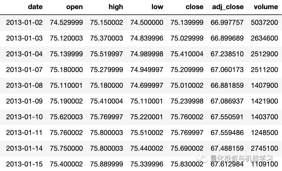
Our goal is to predict the daily adjusted closing price of Vanguard Total Stock Market ETF (VTI) using the data from the previous N days. In this example, we will use VTI’s historical prices from January 2, 2013, to December 28, 2018, for 6 years, as shown in the dataset:

Closing Price

To effectively evaluate the performance of XGBoost, running a prediction on just one date is not enough. Instead, we will perform various predictions on different dates in this dataset and average the results.

To assess the effectiveness of our method, we will use metrics such as Root Mean Square Error (RMSE), Mean Absolute Percentage Error (MAPE), and Mean Absolute Error (MAE). For all metrics, the lower the value, the better the prediction performance. Similar to the previous article, we will use the Last Value method for benchmarking the results.

Exploratory Data Analysis (EDA)

EDA is an important part of machine learning projects, as it helps us gain a good “perception” of the dataset. As we will see below, the EDA process involves creating visualizations to help everyone better understand the dataset.

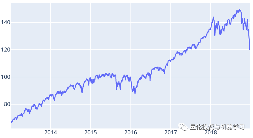
The following figure shows the monthly adjusted closing price’s mean. Based on the dataset, it can be inferred that the values in the later months are higher than those in the earlier months on average.

Month

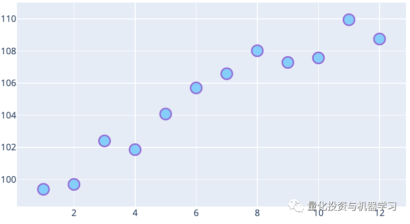
The following figure shows the mean of the adjusted closing price for each day of the month. On average, there is an upward trend, meaning that the prices at the end of the month are higher than in the previous days.

Day

The following figure shows the mean of the adjusted closing price for each day of the week. On average, the adjusted closing prices on Thursday and Friday are higher than those on other days of the week.

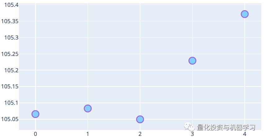
Week

The following heatmap shows the correlation between the adjusted closing prices of the previous few days and the closing price of the current day. It is clear that the closer the adjusted closing price is to the current day, the higher the correlation. Therefore, features related to the adjusted closing prices of the previous 10 days should be used in the predictions.

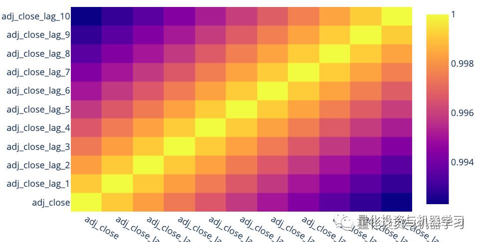
Based on the above EDA, we infer that date-related features may be helpful for the model. Additionally, the adjusted closing prices of the previous 10 days are highly correlated with the target variable. These are important pieces of information we will use in the feature engineering below.

Feature Engineering

Feature engineering is a creative process and one of the most important parts of any machine learning project. To emphasize the importance of feature engineering, Andrew Ng has a great quote worth sharing:

Coming up with features is difficult, time-consuming, and requires expert knowledge. “Applied machine learning” is basically feature engineering.

Andrew Ng, Machine Learning and AI via Brain simulations

In this article, we will generate the following features:

1. Adjusted closing price of the past 10 days

2. Year3. Month4. Week5. Day of Month6. Day of Week7. Day of Year8. Is Month End9. Is Month Start10. Is Quarter End11. Is Quarter Start12. Is Year End13. Is Year Start

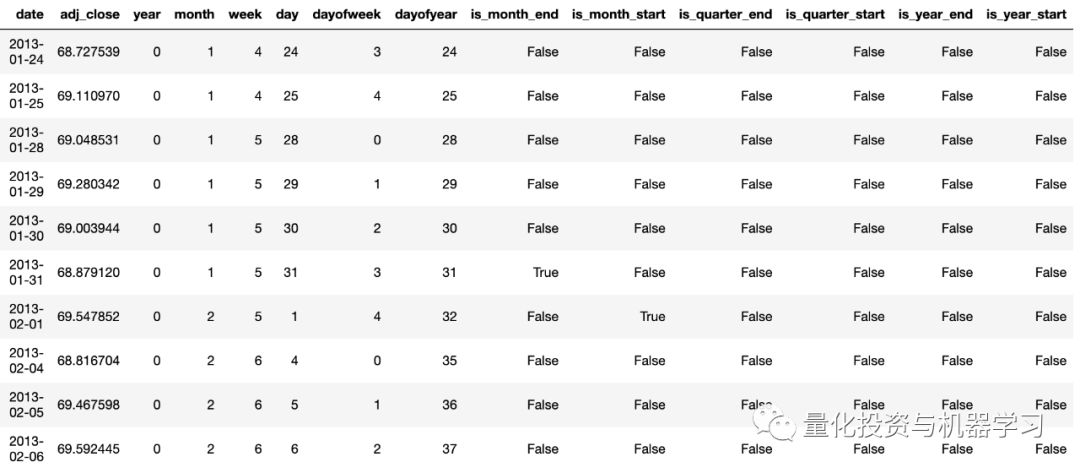
Using the fastai package, it is easy to generate date-related features, such as:

from fastai.tabular import add_datepart

add_datepart(df, 'date', drop=False)
df.drop('Elapsed', axis=1, inplace=True)

After using the above code, the dataframe looks as follows. The column adj_close will be the target column. For brevity, we omit the relevant information of the adjusted closing prices from the past N days.

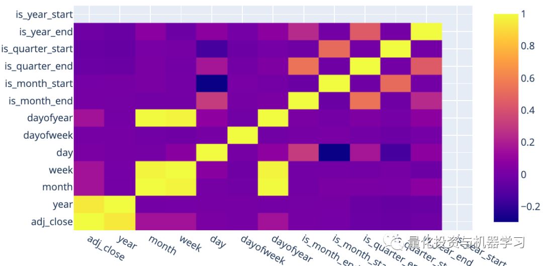
The following heatmap shows the correlation between these features and the target column. The feature year is highly correlated with the adjusted closing price. This is not surprising, as there is an upward trend in our dataset, where higher years correspond to higher adjusted closing prices. Other features do not have high correlations with the target variable. From below, we also find that is_year_start has null values. This is because the first day of each year is never a trading day, so we removed this feature from the model.

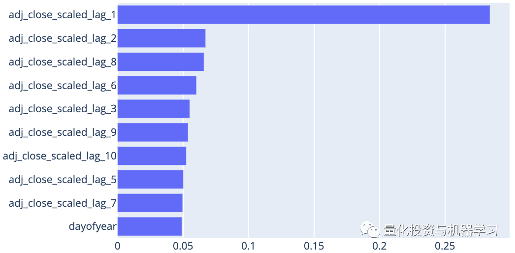
The following bar chart shows the importance scores of the top 10 most important features. This is based on predictions made for January 3, 2017, and the rankings of feature importance may differ for predictions made on other dates. As expected, the adjusted closing price from the previous day is the most important feature.

Training, Validation, and Testing

To make predictions, we need training and validation data. We will use 3 years of data as the training set, which amounts to 756 days, as there are approximately 252 trading days in a year (252*3 = 756). We will use the next year’s data for validation, which amounts to 252 days. In other words, for each prediction made, we need 756 + 252 = 1008 days of data for model training and validation. The model will be trained on the training set, while hyperparameters will be tuned using the validation set.To tune hyperparameters, we will use the moving window validation method.

Below is an example illustrating a training size of 756 days, a validation size of 40 days, and a prediction period of 40 days.

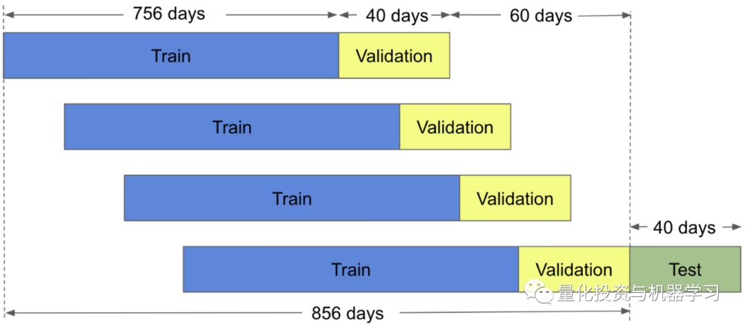
In time series forecasting, it is crucial that training, validation, and testing are conducted in chronological order! Failing to do this will lead to “information leakage” in the model.

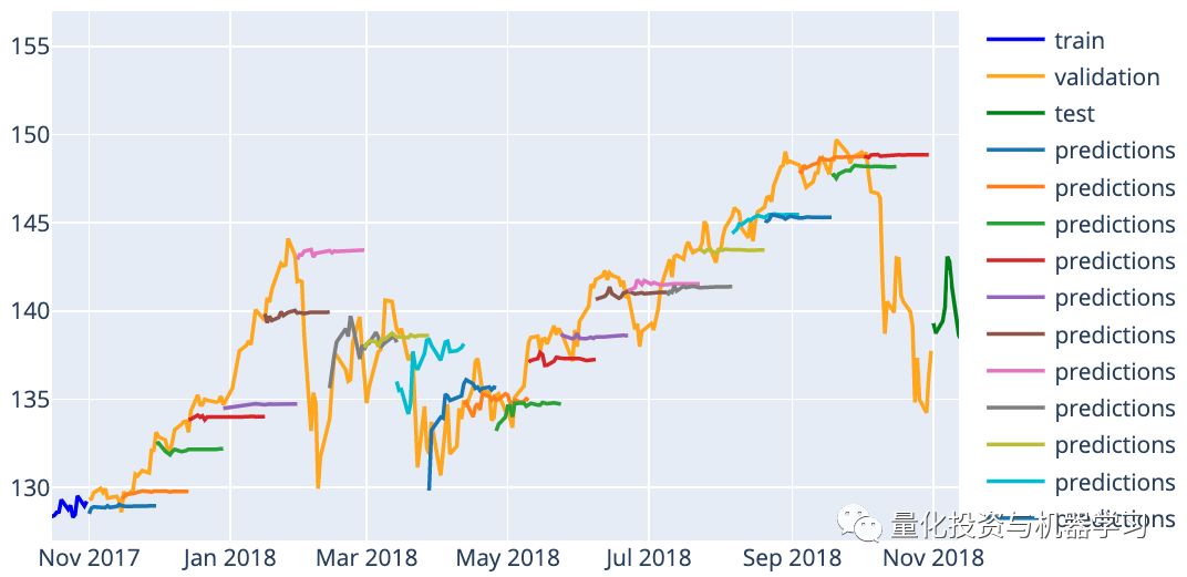
Next, we will use XGBoost to make predictions on our test set for several days, namely:

January 3, 2017, March 6, 2017, May 4, 2017, July 5, 2017, September 1, 2017, November 1, 2017, January 3, 2018, March 6, 2018, May 4, 2018, July 5, 2018, September 4, 2018, November 1, 2018

For the above 12 predictions, we will use a prediction period of 21 days. We will use the 1008 days immediately before the prediction date as the training and validation set (756:252).

Feature Scaling

Feature scaling is important here because, if you look at the above adjusted closing prices, the training and testing sets divided by time will almost always lead to adjusted closing prices being higher than training prices. Specifically, see this article: Rigorous Solutions to 5 Machine Learning Algorithms in Stock Price Prediction (Code + Data)

For each sample’s adjusted closing price group, we will scale it to have a mean of 0 and a variance of 1. For example, if we are predicting for day T, we will take the adjusted closing prices from the last N days (from day T to day T) and adjust them to have a mean of 0 and a variance of 1. The same operation will be performed on lag features across training, validation, and testing sets. Date features are not scaled. We will then use these scaled lag features and date features for prediction. The predicted values will also be scaled, and then we will use their corresponding means and variances to revert them back.

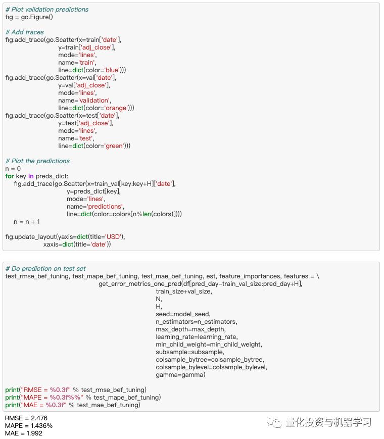
Hyperparameter Tuning

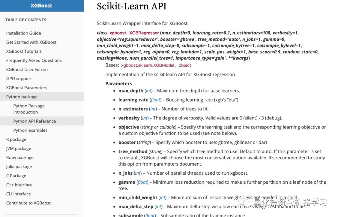
We perform hyperparameter tuning on the validation set. For XGBoost, there are several hyperparameters that can be tuned, including n_estimators, max_depth, learning_rate, min_child_weight, subsample, gamma, colsample_bytree, and colsample_bylevel. For definitions of these hyperparameters, see here:

https://xgboost.readthedocs.io/en/latest/python/python_api.html#module-xgboost.sklearn

To check the effectiveness of hyperparameter tuning, we can look at the predictions for November 1, 2018, on the validation set. The predictions shown below were made without hyperparameter tuning; we simply used the default values from the package:

Below are the predictions on the same validation set after hyperparameter tuning. You can see that the prediction for January 18 is more stable.

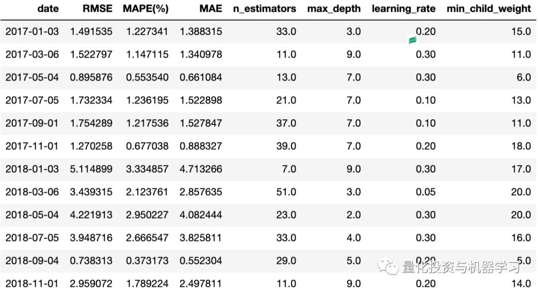
Hyperparameters before and after tuning:

Clearly, the tuned hyperparameters differ significantly from the default values. Additionally, after tuning the RMSE, MAPE, and MAE for validation, the validation results decreased as expected. For example, RMSE dropped from 3.395 to 2.984.

Model Application

After executing the above steps, we are now ready to make predictions on the test set. In this case, our prediction period is 21 days, meaning we need to generate 21 predictions for each prediction. We cannot generate all 21 predictions at once because after generating the prediction for day T, we need to feedback this prediction into our model to generate the prediction for day T+1, and so on, until we obtain all 21 predictions. This is known as recursive prediction. Therefore, we implemented the logic as shown in the flowchart below:

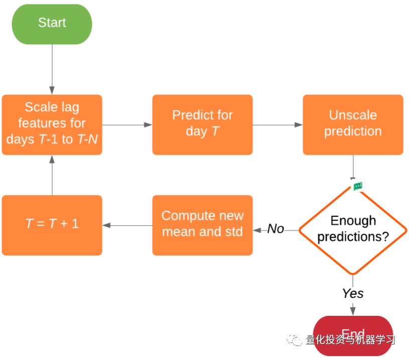
For each day within the prediction range, we need to predict, cancel the prediction scale, calculate the new mean and standard deviation of the last N values, adjust the recent N days’ closing prices, and then predict again.

Results

The following shows the RMSE, MAPE, and MAE for each prediction, along with the corresponding best hyperparameters adjusted using their respective validation sets.

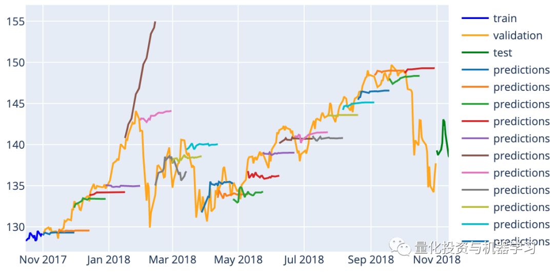
Results of applying XGBoost on the test set using the moving window validation method are shown below:

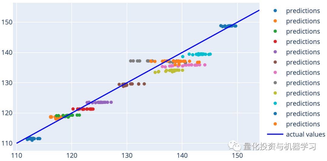
Another way to visualize predictions is to plot each prediction against its actual value. If our predictions were perfect, each prediction should lie on the diagonal line y=x.

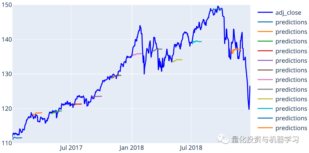
Finally, here are the results of our model compared to the Last Value method:

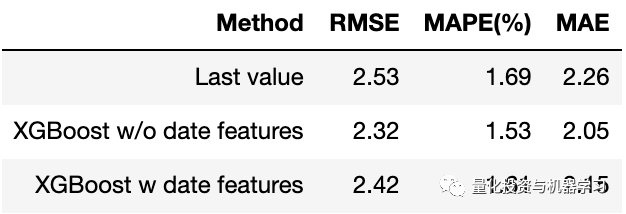
Compared to the Last Value method, using XGBoost with or without date features yields better performance. Interestingly, omitting date features resulted in slightly lower RMSE than including them (2.32 vs. 2.42). As we found earlier, date features have low correlation with the target variable and may not be very helpful for the model.

Partial Code Display

Due to the large amount of code, only a portion is displayed; to obtain the complete code, see the end of the article:

Code Access

In thebackend enter (case-sensitive)

XGBoost_QIML_StockPricePrediction

—End—

The WeChat Official Account for Quantitative Investment and Machine Learning is a vertical platform in the industry focusing onQuant,MFE,CST, AI and other professional fields. The official account has over180,000+ followers from various sectors including public offerings, private equity, brokerage firms, banks, and overseas. It publishes cutting-edge research results and the latest quantitative news daily.Every “Like” you give is our greatest encouragement