My XGBoost Learning Experience and Hands-On Practice

↑↑↑ Follow and “Star” Datawhale

Daily Insights & Monthly Learning Teams, Don’t Miss Out

Datawhale Insights

Author: Li Zuxian, Shenzhen University, Datawhale University Group Member

Zhihu Address: http://www.zhihu.com/people/meng-di-76-92

Today, I will mainly introduce XGBoost, one of the three giants in machine learning ensemble methods. This algorithm has previously shone in machine learning competitions and is a very useful ensemble algorithm.

XGBoost is an optimized distributed gradient boosting library designed for efficiency, flexibility, and portability. It implements machine learning algorithms under the Gradient Boosting framework. XGBoost provides parallel tree boosting (also known as GBDT, GBM), which can quickly and accurately solve many data science problems.

The same code can run in major distributed environments (Hadoop, SGE, MPI) and can solve problems with billions of samples. XGBoost leverages out-of-core computing, enabling data scientists to handle hundreds of millions of sample data on a single machine. Ultimately, these techniques are combined to create an end-to-end system that scales to larger datasets with minimal cluster systems.

Introduction to XGBoost Principles

Starting from scratch, I went through the twists and turns of deriving formulas. Below, I will showcase my handwritten notes on the formulas, hoping to inspire everyone to love machine learning and data mining even more!

XGBoost Formula 1

XGBoost Formula 2

Now, let’s explain the content of the notes in detail:

1. Optimization Objective: Our task is to find a set of trees that minimize OBj. Clearly, this optimization objective OBj can be viewed as a combination of the sample loss and the model complexity penalty.2. Using Additive Training Boosting (Additive Training Boosting)

The core idea is: after training trees, we no longer adjust the previous trees. Thus, the t-th tree can be represented as:

(1). If we train the t-th tree, the objective function becomes:

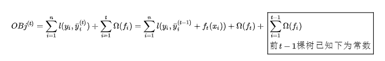
We perform a second-order Taylor expansion on the above equation:

Since the first t-1 trees are known, we have:

(2). We have fully discussed the first half of the loss function, but the second half is just a symbol and not yet defined. Now let’s define : Assume that the t-th tree we are training has T leaf nodes:The output vector of the leaf nodes is represented as follows:

Assuming that represents the mapping from samples to leaf nodes, then .Then we define:

(3). Our objective function ultimately simplifies to:

Once we find the objective function, we need to optimize it:

3. Strategy for Generating Trees:The premise of our previous assumption is that the first t-1 trees are known, so now we will explore how to generate trees. According to the decision tree generation strategy, we need to consider the node that can reduce the loss function the fastest during each split, which we call Gain:

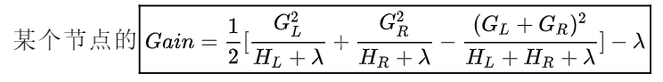
The larger the Gain, the more it indicates that the value of the objective function decreases more after the split. (Because from the equation: the larger it is, the smaller the OBj)

4. Finding Optimal Nodes:

• Exact Greedy Algorithm (Basic Exact Greedy Algorithm)

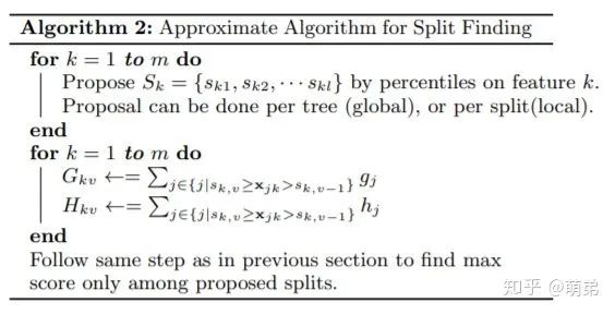
• Approximate Algorithm (Approximate Algorithm)

In the decision tree (CART), we use the exact greedy algorithm (Basic Exact Greedy Algorithm), which sorts all values of all features (which is time and memory-consuming), and then compares the Gini of each point to find the node with the largest change. When the feature is continuous, we discretize the continuous values, taking the average of two points as the split node. As can be seen, the sorting algorithm here takes a lot of time because it needs to traverse all features of the entire sample and sort them!

Therefore, in XGBoost, we use the approximate algorithm (Approximate Algorithm):This algorithm first proposes candidate split points based on the percentiles of the feature distribution, mapping continuous features into buckets divided by these candidate points, aggregating statistical information, and finding the best solution based on the aggregated information. For a certain feature k, the algorithm first finds the candidate set of feature cut points based on the percentiles of the feature distribution , and then divides the values of feature k into buckets according to the set , and finally looks for the best split point based on the accumulated statistics within each bucket.

XGBoost Hands-On Practice:

1. Import Basic Libraries:

# Import basic libraries
import numpy as np
import pandas as pd
import xgboost as xgb
import matplotlib.pyplot as plt
plt.style.use("ggplot")
%matplotlib inline

2. Getting Started with XGBoost Native Library:

import xgboost as xgb  # Import library
# Read in data
dtrain = xgb.DMatrix('demo/data/agaricus.txt.train')   # XGBoost's exclusive data format, but can also use dataframe or ndarray
dtest = xgb.DMatrix('demo/data/agaricus.txt.test')  # # XGBoost's exclusive data format, but can also use dataframe or ndarray
# Specify parameters via map
param = {'max_depth':2, 'eta':1, 'objective':'binary:logistic' }    # Set XGB parameters, passed in dictionary form
num_round = 2     # Use thread count
bst = xgb.train(param, dtrain, num_round)   # Train
# Make prediction
preds = bst.predict(dtest)   # Predict

3. XGBoost Parameter Settings(Names in parentheses correspond to sklearn interface parameter names)

XGBoost parameters are divided into three categories:

1. General Parameters

• booster: Which weak learner to train, default is gbtree, options are gbtree, gblinear or dart

• nthread: Number of parallel threads used to run XGBoost, default is maximum available threads

• verbosity: Level of detail of printed messages. Valid values are 0 (silent), 1 (warning), 2 (info), 3 (debug).

• Tree Booster Parameters:

• eta (learning_rate): learning_rate, shrinkage step to prevent overfitting during updates, default = 0.3, range: [0,1]; typical values are generally set to: 0.01-0.2

• gamma (min_split_loss): default = 0, when splitting nodes, the reduction in the loss function must be greater than or equal to gamma for the node to split; the larger the gamma value, the more conservative the algorithm, making it less likely to overfit, but performance may not be guaranteed, requiring balance. Range: [0, ∞]

• max_depth: default = 6, maximum depth of a tree. Increasing this value makes the model more complex and more likely to overfit. Range: [0, ∞]

• min_child_weight: default = 1, if the sum of sample weights of newly split nodes is less than min_child_weight, stop splitting. This can help reduce overfitting, but cannot be too high, as it may lead to underfitting. Range: [0, ∞]

• max_delta_step: default = 0, maximum incremental step allowed for each leaf output. If this value is set to 0, it means no constraints. If set to a positive value, it can help make update steps more conservative. This parameter is generally not needed, but it may help in logistic regression when classes are extremely unbalanced. Setting it to a value between 1-10 may help control updates. Range: [0, ∞]

• subsample: default = 1, sampling rate of samples used to build each tree; if set to 0.5, XGBoost will randomly select half of the samples as the training set. Range: (0,1]

• sampling_method: default = uniform, method used for sampling training instances.

• uniform: equal probability of selection for each training instance. Typically, setting subsample >= 0.5 yields good results.

• gradient_based: the probability of selection for each training instance is proportional to the absolute value of the regularized gradient, specifically , subsample can be set as low as 0.1 without losing model accuracy.

• colsample_bytree: default = 1, column sampling rate, i.e., feature sampling rate. Range: (0,1]

• lambda (reg_lambda): default = 1, L2 regularization weight. Increasing this value makes the model more conservative.

• alpha (reg_alpha): default = 0, L1 regularization term for weights. Increasing this value makes the model more conservative.

• tree_method: default = auto, tree construction algorithm used in XGBoost.

• auto: uses a heuristic to select the fastest method.

• For small datasets, exact will use the exact greedy algorithm.

• For larger datasets, approx will choose the approximate algorithm. It is recommended to try hist, gpu_hist for potentially higher performance with large datasets. (gpu_hist) supports external memory.

• exact: exact greedy algorithm. Enumerates all candidate points for splits.

• approx: uses quantiles and gradient histograms for the approximate greedy algorithm.

• hist: faster histogram-optimized approximate greedy algorithm. (LightGBM also uses histogram algorithms)

• gpu_hist: implementation of GPU hist algorithm.

• scale_pos_weight: controls the balance of positive and negative weights, which is useful for imbalanced classes. In Kaggle competitions, it is generally set to sum(negative instances) / sum(positive instances), and in cases of high class imbalance, setting this parameter greater than 0 can speed up convergence.

• num_parallel_tree: default = 1, number of parallel trees constructed during each iteration. This option is used to support enhanced random forests.

• monotone_constraints: constraints for variable monotonicity, which can be used in cases where there is a very strong prior belief that the true relationship has a certain quality, to improve the model’s predictive performance. (e.g., params_constrained[‘monotone_constraints’] = “(1,-1)”, (1,-1) tells XGBoost to impose an increasing constraint on the first predictor variable and a decreasing constraint on the second predictor variable.)

Linear Booster Parameters:

• lambda (reg_lambda): default = 0, L2 regularization weight. Increasing this value makes the model more conservative. Normalized by the number of training examples.

• alpha (reg_alpha): default = 0, L1 regularization term for weights. Increasing this value makes the model more conservative. Normalized by the number of training examples.

• updater: default = shotgun.

• shotgun: parallel coordinate descent algorithm based on the shotgun algorithm. Uses “hogwild” parallelism, resulting in uncertain solutions each time it runs.

• coord_descent: ordinary coordinate descent algorithm. Also multithreaded, but still produces deterministic solutions.

• feature_selector: default = cyclic. Feature selection and sorting method

• cyclic: achieved by looping through one feature at a time.

• shuffle: similar to cyclic, but with random feature transformations before each update.

• random: a random (with replacement) feature selector.

• greedy: selects the feature with the largest gradient. (Greedy selection)

• thrifty: approximate greedy feature selection (similar to greedy)

• top_k: number of most important features to select (within greedy and thrifty)

There are two types of general parameters for boosters, as tree performance is much better than linear regression, so we rarely use linear regression.

2. Task Parameters

• objective: default = reg:squarederror, indicating minimum squared error.

• reg:squarederror, minimum squared error.

• reg:squaredlogerror, log squared loss.

• reg:logistic, logistic regression

• reg:pseudohubererror, regression using pseudo-Huber loss, which is a twice differentiable choice of absolute loss.

• binary:logistic, logistic regression for binary classification, outputs probabilities.

• binary:logitraw: output scores before logistic transformation for binary classification.

• binary:hinge: hinge loss for binary classification. This predicts either 0 or 1, rather than producing probabilities. (SVM uses hinge loss function)

• count:poisson – Poisson regression for count data, output mean of Poisson distribution.

• survival:cox: Cox regression for censored survival time data (negative values are treated as correct survival times).

• survival:aft: accelerated failure time model for checking survival time data.

• aft_loss_distribution: probability density function used in survival:aft and aft-nloglik metrics.

• multi:softmax: sets XGBoost to use softmax objective for multi-class classification, num_class (number of classes) must also be set

• multi:softprob: same as softmax, but outputs a vector that can be reshaped into a matrix. The result includes predicted probabilities for each data point belonging to each class.

• rank:pairwise: uses LambdaMART for pairwise ranking, minimizing pairwise loss.

• rank:ndcg: uses LambdaMART for list ranking, maximizing normalized discounted cumulative gain (NDCG).

• rank:map: uses LambdaMART for average ranking, maximizing mean average precision (MAP).

• reg:gamma: gamma regression using log link. Output is the mean of the gamma distribution.

• reg:tweedie: Tweedie regression using log link.

• Custom loss functions and evaluation metrics:

• eval_metric: evaluation metric for validation data, default metrics will be assigned based on the objective (RMSE for regression, classification error, mean average precision for ranking), users can add multiple evaluation metrics

• rmse, root mean square error; rmsle: root mean square logarithmic error; mae: mean absolute error; mphe: mean pseudo-Huber error; logloss: negative log likelihood; error: binary classification error rate;

• merror: multi-class classification error rate; mlogloss: multi-class logloss; auc: area under the curve; aucpr: area under the PR curve; ndcg: normalized cumulative discount; map: mean average precision;

• seed: random seed, [default = 0].

This parameter is used to control the ideal optimization target and the measurement method for each step’s results.

3. Command Line Parameters

We won’t discuss this, as the command line console version is rarely used

4. XGBoost Parameter Tuning Instructions:

General steps for parameter tuning:

• 1. Determine initial values for (larger) learning rate and boosting parameters

• 2. Tune max_depth and min_child_weight parameters

• 3. Tune gamma parameter

• 4. Tune subsample and colsample_bytree parameters

• 5. Tune regularization parameter alpha

• 6. Reduce learning rate and use more decision trees

5. Detailed Guide to XGBoost:

1). Install XGBoost

# Method 1:
pip3 install xgboost
# Method 2:
pip install xgboost

2). Data Interfaces (XGBoost can process data in DMatrix format)

# 1. LibSVM text format file
dtrain = xgb.DMatrix('train.svm.txt')
dtest = xgb.DMatrix('test.svm.buffer')
# 2. CSV file (cannot contain categorical text variables, if text variables exist, preprocess them like one-hot)
dtrain = xgb.DMatrix('train.csv?format=csv&label_column=0')
dtest = xgb.DMatrix('test.csv?format=csv&label_column=0')
# 3. NumPy array
data = np.random.rand(5, 10)  # 5 entities, each contains 10 features
label = np.random.randint(2, size=5)  # binary target
dtrain = xgb.DMatrix(data, label=label)
# 4. scipy.sparse array
csr = scipy.sparse.csr_matrix((dat, (row, col)))
dtrain = xgb.DMatrix(csr)
# pandas dataframe
dataframe = pandas.DataFrame(np.arange(12).reshape((4,3)), columns=['a', 'b', 'c'])
label = pandas.DataFrame(np.random.randint(2, size=4))
dtrain = xgb.DMatrix(data, label=label)

The author recommends: first save to XGBoost binary file to speed up loading, then load it back

# 1. Save DMatrix to XGBoost binary file
dtrain = xgb.DMatrix('train.svm.txt')
dtrain.save_binary('train.buffer')
# 2. Missing values can be replaced with defaults in DMatrix constructor:
dtrain = xgb.DMatrix(data, label=label, missing=-999.0)
# 3. Weights can be set when needed:
w = np.random.rand(5, 1)
dtrain = xgb.DMatrix(data, label=label, missing=-999.0, weight=w)

3). Parameter Setting Methods:

# Load and process data
df_wine = pd.read_csv('https://archive.ics.uci.edu/ml/machine-learning-databases/wine/wine.data',header=None)
df_wine.columns = ['Class label', 'Alcohol','Malic acid', 'Ash','Alcalinity of ash','Magnesium', 'Total phenols',                   'Flavanoids', 'Nonflavanoid phenols','Proanthocyanins','Color intensity', 'Hue','OD280/OD315 of diluted wines','Proline']
df_wine = df_wine[df_wine['Class label'] != 1]  # drop 1 class
y = df_wine['Class label'].values
X = df_wine[['Alcohol','OD280/OD315 of diluted wines']].values
from sklearn.model_selection import train_test_split  # Split training and testing sets
from sklearn.preprocessing import LabelEncoder   # Encode categorical variables
le = LabelEncoder()
y = le.fit_transform(y)
X_train,X_test,y_train,y_test = train_test_split(X,y,test_size=0.2,random_state=1,stratify=y)
dtrain = xgb.DMatrix(X_train, label=y_train)
dtest = xgb.DMatrix(X_test)
# 1. Booster parameters
params = {    'booster': 'gbtree',    'objective': 'multi:softmax',  # Multi-class problem    'num_class': 10,               # Number of classes, used with multisoftmax    'gamma': 0.1,                  # Parameter for controlling whether to prune later, the larger the more conservative, generally around 0.1, 0.2.    'max_depth': 12,               # Depth of the tree, the larger the more likely to overfit    'lambda': 2,                   # Parameter controlling the weight of model complexity, the larger the less likely to overfit.    'subsample': 0.7,              # Randomly sample training samples    'colsample_bytree': 0.7,       # Column sampling during tree generation    'min_child_weight': 3,    'silent': 1,                   # Set to 1 for no run information output, best set to 0.    'eta': 0.007,                  # Similar to learning rate    'seed': 1000,    'nthread': 4,                  # CPU thread count    'eval_metric':'auc'}
plst = params.items()
# evallist = [(dtest, 'eval'), (dtrain, 'train')]   # Specify validation set

4). Training

# 2. Training
num_round = 10
bst = xgb.train( plst, dtrain, num_round)
#bst = xgb.train( plst, dtrain, num_round, evallist )

5). Save Model

# 3. Save model
bst.save_model('0001.model')
# dump model
bst.dump_model('dump.raw.txt')
# dump model with feature map
#bst.dump_model('dump.raw.txt', 'featmap.txt')

6). Load Saved Model

# 4. Load saved model: bst = xgb.Booster({'nthread': 4})  # init model
bst.load_model('0001.model')  # load data

7). Set Early Stopping Mechanism

# 5. You can also set an early stopping mechanism (requires setting validation set)
train(..., evals=evals, early_stopping_rounds=10)

8). Prediction

# 6. Prediction
ypred = bst.predict(dtest)

9). Plotting

# 1. Plot importance
xgb.plot_importance(bst)
# 2. Plot output tree
#xgb.plot_tree(bst, num_trees=2)
# 3. Use xgboost.to_graphviz() to convert target tree to graphviz
#xgb.to_graphviz(bst, num_trees=2)

6. Practical Cases:

1). Classification Case

from sklearn.datasets import load_iris
import xgboost as xgb
from xgboost import plot_importance
from matplotlib import pyplot as plt
from sklearn.model_selection import train_test_split
from sklearn.metrics import accuracy_score   # Accuracy
# Load sample dataset
iris = load_iris()
X,y = iris.data,iris.target
X_train, X_test, y_train, y_test = train_test_split(X, y, test_size=0.2, random_state=1234565) # Split dataset
# Algorithm parameters
params = {    'booster': 'gbtree',    'objective': 'multi:softmax',    'num_class': 3,    'gamma': 0.1,    'max_depth': 6,    'lambda': 2,    'subsample': 0.7,    'colsample_bytree': 0.75,    'min_child_weight': 3,    'silent': 0,    'eta': 0.1,    'seed': 1,    'nthread': 4,}
plst = params.items()
dtrain = xgb.DMatrix(X_train, y_train) # Generate dataset format
num_rounds = 500
model = xgb.train(plst, dtrain, num_rounds) # Train xgboost model
# Predict on test set
dtest = xgb.DMatrix(X_test)
y_pred = model.predict(dtest)
# Calculate accuracy
accuracy = accuracy_score(y_test,y_pred)
print("accuracy: %.2f%%" % (accuracy*100.0))
# Show important features
plot_importance(model)
plt.show()

2). Regression Case

import xgboost as xgb
from xgboost import plot_importance
from matplotlib import pyplot as plt
from sklearn.model_selection import train_test_split
from sklearn.datasets import load_boston
from sklearn.metrics import mean_squared_error
# Load dataset
boston = load_boston()
X,y = boston.data,boston.target
# XGBoost training process
X_train, X_test, y_train, y_test = train_test_split(X, y, test_size=0.2, random_state=0)
params = {    'booster': 'gbtree',    'objective': 'reg:squarederror',    'gamma': 0.1,    'max_depth': 5,    'lambda': 3,    'subsample': 0.7,    'colsample_bytree': 0.7,    'min_child_weight': 3,    'silent': 1,    'eta': 0.1,    'seed': 1000,    'nthread': 4,}
dtrain = xgb.DMatrix(X_train, y_train)
num_rounds = 300
plst = params.items()
model = xgb.train(plst, dtrain, num_rounds)
# Predict on test set
dtest = xgb.DMatrix(X_test)
ans = model.predict(dtest)
# Show important features
plot_importance(model)
plt.show()

7. XGBoost Parameter Tuning (combined with sklearn grid search)

import xgboost as xgb
import pandas as pd
from sklearn.model_selection import train_test_split
from sklearn.model_selection import GridSearchCV
from sklearn.metrics import roc_auc_score
iris = load_iris()
X,y = iris.data,iris.target
col = iris.target_names
train_x, valid_x, train_y, valid_y = train_test_split(X, y, test_size=0.3, random_state=1)   # Split training and validation sets
parameters = {              'max_depth': [5, 10, 15, 20, 25],              'learning_rate': [0.01, 0.02, 0.05, 0.1, 0.15],              'n_estimators': [500, 1000, 2000, 3000, 5000],              'min_child_weight': [0, 2, 5, 10, 20],              'max_delta_step': [0, 0.2, 0.6, 1, 2],              'subsample': [0.6, 0.7, 0.8, 0.85, 0.95],              'colsample_bytree': [0.5, 0.6, 0.7, 0.8, 0.9],              'reg_alpha': [0, 0.25, 0.5, 0.75, 1],              'reg_lambda': [0.2, 0.4, 0.6, 0.8, 1],              'scale_pos_weight': [0.2, 0.4, 0.6, 0.8, 1]}
xlf = xgb.XGBClassifier(max_depth=10,            learning_rate=0.01,            n_estimators=2000,            silent=True,            objective='multi:softmax',            num_class=3 ,            nthread=-1,            gamma=0,            min_child_weight=1,            max_delta_step=0,            subsample=0.85,            colsample_bytree=0.7,            colsample_bylevel=1,            reg_alpha=0,            reg_lambda=1,            scale_pos_weight=1,            seed=0,            missing=None)
gs = GridSearchCV(xlf, param_grid=parameters, scoring='accuracy', cv=3)
gs.fit(train_x, train_y)
print("Best score: %0.3f" % gs.best_score_)
print("Best parameters set: %s" % gs.best_params_ )

This article's electronic version can be obtained by replying XGBoost in the background

👇 Click to read the original text and follow the author