
XGBoost is the most famous algorithm for handling different types of tabular data, with LightGBM and Catboost released to address its shortcomings. On September 12, XGBoost released the new version 2.0. This article will not only introduce the complete history of XGBoost but also discuss the new mechanisms and updates.
This is a long article, as we will first start with gradient-boosted decision trees.
Tree-based methods, such as decision trees, random forests, and the extended XGBoost, excel at handling tabular data because their hierarchical structure is inherently good at modeling the common hierarchical relationships found in tabular formats. They are particularly effective at automatically detecting and integrating complex nonlinear interactions between features. Additionally, these algorithms are robust to the scale of input features, allowing them to perform well on raw datasets without the need for normalization.
Another important point is that they provide the advantage of natively handling categorical variables, bypassing the need for preprocessing techniques like one-hot encoding, although XGBoost usually still requires numerical encoding.
Moreover, tree-based models can be easily visualized and interpreted, further increasing their appeal, especially when understanding the structure of tabular data. By leveraging these inherent advantages, tree-based methods—especially advanced methods like XGBoost—are well-suited to tackle various challenges in data science, particularly when dealing with tabular data.
Decision Trees
In stricter mathematical language, a decision tree represents a function T:X→Y, where X is the feature space and Y can be continuous values (in the case of regression) or class labels (in the case of classification). We can represent the data distribution as D and the true function f:X→Y. The goal of the decision tree is to find T(x) that is very close to f(x), ideally under the probability distribution D.
Loss Function
The risk R associated with the tree T relative to f is expressed as the expected value of the loss function between T(x) and f(x):
The primary objective of building a decision tree is to create a model that generalizes well to new, unseen data. Ideally, we know the true distribution D of the data, allowing us to directly compute the risk or expected loss of any candidate decision tree. However, in practice, the true distribution is unknown.
Thus, we rely on a subset of the available data to make decisions. This is where the concept of heuristic methods comes into play.
Gini Index
The Gini index is a measure of impurity that quantifies the degree of mixing of classes in a given node. The formula for the Gini index G at a given node t is:
Where p_i is the proportion of samples in class i at node t, and c is the number of classes.
The Gini index ranges from 0 to 0.5, where lower values indicate that the node is purer (i.e., primarily containing samples from one class).
Gini Index or Information Gain?
The Gini index and Information Gain are both metrics for quantifying the “usefulness” of features that distinguish different classes. Essentially, they provide a way to evaluate how well a feature splits the data into classes. By selecting the feature that reduces impurity the most (lowest Gini index or highest Information Gain), a heuristic decision can be made, which is the best local choice at this step of tree growth.
Overfitting and Pruning
Decision trees can also overfit, especially when they are deep, capturing noise in the data. There are two main strategies to address this issue:
- Splitting: As the tree grows, continuously monitor its performance on the validation dataset. If performance begins to decline, this is a signal to stop growing the tree.
- Post-pruning: After the tree has fully grown, prune nodes that do not provide much predictive power. This is usually done by removing nodes and checking if it reduces validation accuracy. If not, prune the node.
Finding the optimal risk-minimizing tree is challenging because we do not know the true data distribution D. Therefore, we can only use heuristic methods, such as the Gini index or Information Gain, to locally optimize the tree based on the available data, while careful splitting and pruning techniques help manage model complexity and avoid overfitting.
Random Forests
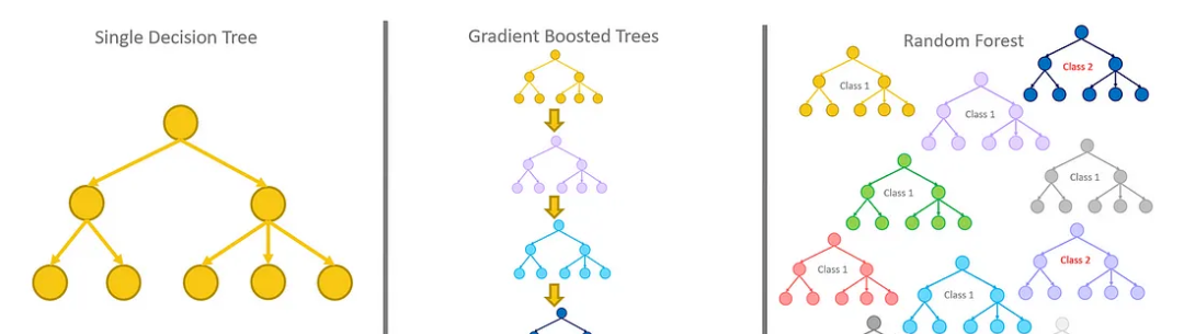
A random forest is an ensemble of decision trees T_1, T_2, …, T_n, where each decision tree T_i:X→Y maps the input feature space X to output Y, which can be continuous values (regression) or class labels (classification).
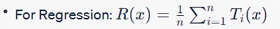
The random forest ensemble defines a new function R:X→Y, which performs a majority vote (classification) or averaging (regression) over the outputs of all individual trees, mathematically expressed as:

Like decision trees, random forests also aim to approximate the true function f:X→Y under the probability distribution D. In practice, D is usually unknown, so heuristic methods are necessary to construct individual trees.
The risk R_RF associated with random forests relative to f is the expected value of the loss function between R(x) and f(x). Given that R is a collection of T, the risk is typically lower than the risk associated with individual trees, which aids generalization:
Overfitting and Bagging
Compared to a single decision tree, random forests are less prone to overfitting, thanks to bagging and feature randomization, which creates diversity among trees. Risks are averaged over multiple trees, making the model more resilient to noise in the data.
Bagging in random forests achieves multiple objectives: it reduces overfitting by averaging predictions across different trees, with each tree trained on different bootstrap samples, making the model more resilient to noise and fluctuations in the data. This also reduces variance, leading to more stable and accurate predictions. The ensemble of trees can capture different aspects of the data, improving the model’s generalization to unseen data. It can also provide higher robustness, as correct predictions from other trees often offset errors from individual trees. This technique can enhance the representation of minority classes in imbalanced datasets, making the ensemble more suitable for such challenges.
Random forests adopt heuristic methods at the individual tree level but mitigate some limitations through ensemble learning, thus providing a balance between fitting and generalization. Techniques like bagging and feature randomization further reduce risk and enhance model robustness.
Gradient Boosted Decision Trees
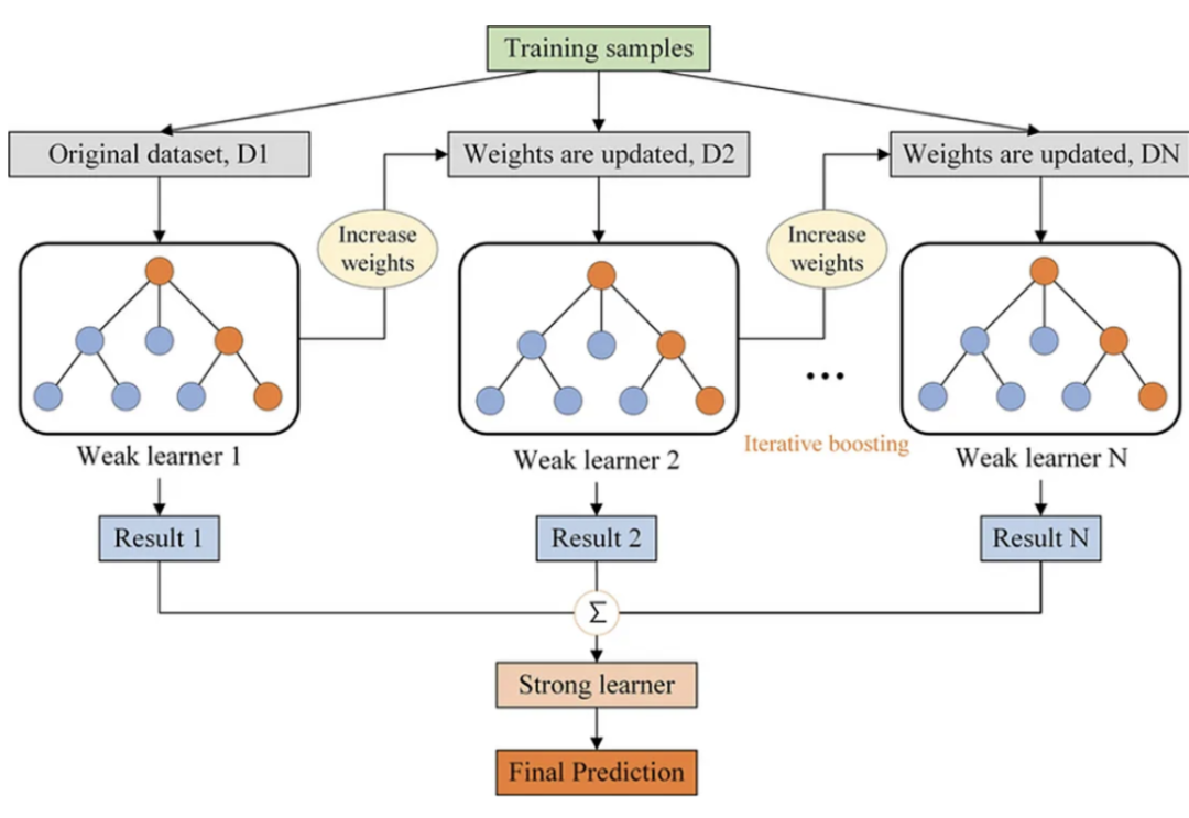
Gradient Boosted Decision Trees (GBDT) are also an ensemble method that constructs a strong predictive model by iteratively adding decision trees, with each new tree aimed at correcting the errors of the existing ensemble. Mathematically, GBDT also represents a function T:X→Y, but instead of finding a single T(X), it forms a sequence of weak learners t_1(X), t_2(X), … that work together to approximate the true function f(X). Unlike random forests, which build trees independently through bagging, GBDT constructs trees in sequence, using gradient descent to minimize the difference between predicted and true values, typically represented through a loss function.
In GBDT, after building each tree and making predictions, the residuals (or errors) between the predicted values and the actual values are computed. These residuals essentially represent a form of gradient—indicating how the loss function changes with respect to its parameters. A new tree is then fitted to these residuals instead of the original outcome variable, effectively taking a “step” to utilize gradient information to minimize the loss function. This process is repeated, iteratively improving the model.
The term “gradient” implies the use of gradient descent optimization to guide the sequential construction of trees, aimed at continuously minimizing the loss function, thereby making the model more predictive.
Why Is It Better Than Decision Trees and Random Forests?
- Reducing Overfitting: Like random forests, GBDT also avoids overfitting, but it does so by constructing shallow trees (weak learners) and optimizing the loss function instead of averaging or voting.
- High Efficiency: GBDT focuses on difficult-to-classify instances, adapting more to the problem areas of the dataset. This can make it more effective in classification performance compared to random forests, which treat all instances equally.
- Optimizing Loss Function: Unlike heuristic methods (such as the Gini index or Information Gain), the loss function in GBDT is optimized during training, allowing for a more precise fit to the data.
- Better Performance: When the right hyperparameters are chosen, GBDT often outperforms random forests, especially in situations requiring very precise models where computational cost is not a major concern.
- Flexibility: GBDT can be used for both classification and regression tasks, and it is easier to optimize since you can directly minimize the loss function.
Problems Addressed by Gradient Boosted Decision Trees
High Bias of Single Trees: GBDT achieves better performance than single trees by iteratively correcting the errors of single trees.
Model Complexity: Random forests are designed to reduce model variance, while GBDT provides a good balance between bias and variance, often yielding better overall performance.
Gradient Boosted Decision Trees have advantages in performance, adaptability, and optimization over decision trees and random forests. They are particularly useful when high predictive accuracy is required and computational resources are available to fine-tune the model.
XGBoost
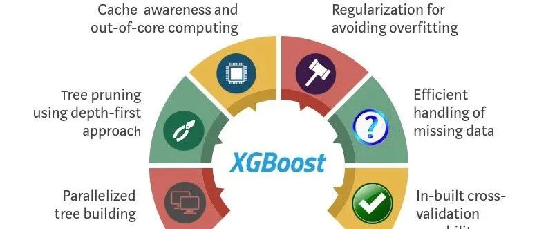
In discussions about tree-based ensemble methods, the focus often falls on the standard advantages: robustness to outliers, ease of interpretation, etc. However, XGBoost has other features that make it stand out and provide advantages in many scenarios.
Computational Efficiency
Typically, discussions around XGBoost focus on its predictive capabilities. What is often less emphasized is its computational efficiency, especially in parallel and distributed computing. The algorithm utilizes features and data points to parallelize tree structures, enabling it to handle larger datasets and run faster than traditional implementations.
Handling Missing Data
XGBoost employs a unique approach to handle missing values. Unlike other models that typically require separate preprocessing steps, XGBoost can handle missing data internally. During training, the algorithm finds the best imputation value (or direction of movement in the tree structure) for missing values and stores it for future predictions. This means that XGBoost’s approach to handling missing data is adaptive and can vary by node, allowing for more nuanced treatment of these values.
Regularization
While boosting algorithms are inherently prone to overfitting, especially with noisy data, XGBoost incorporates L1 (Lasso) and L2 (Ridge) regularization directly into the objective function during training. This approach provides an additional mechanism to constrain the complexity of individual trees rather than simply limiting their depth, thereby improving generalization.
Sparsity
XGBoost is designed to efficiently handle sparse data, not just dense matrices. In fields such as natural language processing using bag-of-words or TF-IDF representations, the sparsity of the feature matrix can pose significant computational challenges. XGBoost utilizes compressed memory-efficient data structures, and its algorithm is designed to efficiently traverse sparse matrices.
Hardware Optimization
While rarely discussed, hardware optimization is a highlight of XGBoost. It optimizes memory efficiency and computation speed on CPUs and supports training models on GPUs, further accelerating the training process.
Feature Importance and Model Interpretability
Most ensemble methods provide feature importance metrics, including random forests and standard gradient boosting. However, XGBoost offers a more comprehensive set of feature importance metrics, including gain, frequency, and coverage, allowing for a more detailed interpretation of the model. This is crucial when it is important to understand which features are significant and how they contribute to predictions.
Early Stopping Strategy
Another feature that is not often discussed is early stopping. Techniques such as careful splitting and pruning are used to prevent overfitting, while XGBoost provides a more automated approach. Once the model’s performance on the validation dataset stops improving, the training process can be halted, saving computational resources and time.
Handling Categorical Variables
While tree-based algorithms can handle categorical variables well, XGBoost employs a unique method. It does not require one-hot encoding or ordinal encoding, allowing categorical variables to remain intact. XGBoost’s treatment of categorical variables is more nuanced than simple binary splits, capturing complex relationships without additional preprocessing.
The unique features of XGBoost make it not only a state-of-the-art machine learning algorithm in terms of predictive accuracy but also an efficient and customizable algorithm. It can handle the complexities of real-world data, such as missing values, sparsity, and multicollinearity, while being computationally efficient and providing detailed interpretability, making it a valuable tool for various data science tasks.
What’s New in XGBoost 2.0?
Above is some background knowledge we’ve introduced, and now we will discuss several interesting updates provided by XGBoost 2.0 that may impact the machine learning community and research.
Multi-Objective Trees with Vector Leaf Outputs
Earlier, we discussed how decision trees in XGBoost use second-order Taylor expansion to approximate the objective function. In 2.0, it transitions to multi-objective trees with vector leaf outputs. This enables the model to capture correlations between objectives, a feature that is especially useful for multitask learning. It aligns with XGBoost’s emphasis on regularization to prevent overfitting, now allowing regularization to work across objectives.
Device Parameters
XGBoost can use different hardware. In version 2.0, XGBoost simplifies the device parameter settings. The “device” parameter replaces multiple device-related parameters, such as gpu_id, gpu_hist, etc., making it easier to switch between CPU and GPU.
Hist as the Default Tree Method
XGBoost allows for different types of tree-building algorithms. Version 2.0 sets ‘hist’ as the default tree method, which may improve performance consistency. This can be seen as XGBoost doubling the efficiency of histogram-based methods.
GPU-Based Approximate Tree Methods
The new version of XGBoost also provides initial support for “approximate” tree methods using GPUs. This can be seen as an attempt to further leverage hardware acceleration, consistent with XGBoost’s focus on computational efficiency.
Memory and Cache Optimization
2.0 continues this trend by providing a new parameter (max_cached_hist_node) to control the size of the CPU cache for histograms and improving external memory support by replacing file IO logic with memory mapping.
Learning-to-Rank Enhancements
Considering XGBoost’s strong performance in various ranking tasks, version 2.0 introduces many features to improve learning to rank, such as new parameters and methods for pairwise construction and support for custom gain functions, etc.
Support for New Quantile Regression
Combining quantile regression, XGBoost can adapt well to different problem domains and loss functions. It also adds a useful tool for estimating uncertainty in predictions.
Conclusion
It has been a while since I dealt with tabular data, so I haven’t paid much attention to XGBoost, but I recently discovered that version 2.0 has been updated, which feels great.
XGBoost version 2.0 is a comprehensive update that continues to build on the existing advantages of scalability, efficiency, and flexibility while introducing features that can pave the way for new applications and research opportunities.
For those interested, check out the official updates: https://github.com/dmlc/xgboost/releases