

Top Quantitative Self-Media in the Industry
Author: Smith Translated by: Fang’s Mantou
1
Introduction
Using machine learning to predict the next period’s price or direction based on stock prices is not new, and it does not yield any meaningful predictions. In this article, we will break down the time series data of a series of assets into a simple classification problem to see if machine learning models can better predict the direction of the next cycle. The goal and strategy is to invest in one asset daily. The asset will be the one in which the machine learning model is most confident that the stock price will rise during the next period
2
Importing Related Libraries
require(PerformanceAnalytics)
library(data.table)
library(dplyr)
library(tibble)
library(TTR)
library(tidyr)
library(tidyquant)
library(tsfeatures)
library(rsample)
library(purrr)
library(stringr)
library(tibbletime) # tsibble clashes with the base R index() function
library(xgboost)
library(rvest)
Predefine some initialization objects and set the stock codes of the companies we want to download. We randomly selected 30 stocks from the S&P 500.
set.seed(1234)
##########################################################

Scale_Me <- function(x){
  (x - mean(x, na.rm = TRUE)) / sd(x, na.rm = TRUE)
}

###########################################################

start_date <- "2017-01-01"
end_date <- "2020-01-01"

url <- "https://en.wikipedia.org/wiki/List_of_S%26P_500_companies"
symbols <- url %>%
  read_html() %>%
  html_nodes(xpath = '//*[@id="constituents"]') %>%
  html_table() %>%
  .[[1]] %>%
  filter(!str_detect(Security, "Class A|Class B|Class C")) %>%     # Removes firms with Class A, B & C shares
  sample_n(30) %>%
  pull(Symbol)


#symbols <- c(
#  'GOOG', 'MSFT', 'HOG', 'AAPL', 'FB'
#  'AMZN', 'EBAY', 'IBM', 'NFLX', 'NVDA',
#  'TWTR', 'WMT', 'XRX', 'INTC', 'HPE'
# )
3
Data
Download the data and store it in a new environment.
dataEnv <- new.env()
getSymbols(symbols,
           from = start_date,
           to = end_date,
           #src = "yahoo",
           #adjust = TRUE,
           env = dataEnv)
##  [1] "LEG"  "NLSN" "SLB"  "CHTR" "C"    "REGN" "CCI"  "SYK"  "ROP"  "RL"
## [11] "CERN" "CMG"  "GS"   "CAT"  "MSI"  "BR"   "VRSK" "PNC"  "KEYS" "PHM"
## [21] "FB"   "BKR"  "ABMD" "WYNN" "DG"   "ADI"  "GL"   "TSCO" "FLS"  "CDW"
Once the data is downloaded and stored in the new environment, we will clean the data, put all lists into a single data frame, calculate the daily returns of each asset, and create an upward or downward direction, which will be what the classification model tries to predict.
df <- eapply(dataEnv, function(x){
  as.data.frame(x) %>%
    rename_all(function(n){
      gsub("^(\w+)\.", "", n, perl = TRUE)
    }
    ) %>%
    rownames_to_column("date")
}) %>%
  rbindlist(idcol = TRUE) %>%
  mutate(date = as.Date(date)) %>%
  group_by(.id) %>%
  tq_mutate(
    select = Adjusted,
    mutate_fun = periodReturn,
    period = "daily",
    type = "arithmetic"
  ) %>%
  mutate(
    Adj_lag = lag(Adjusted),
    chng_Adj = ifelse(Adjusted > Adj_lag, 1, 0)
  ) %>%
  select("date", ".id", "Adjusted", "daily.returns", "chng_Adj", "Open", "High", "Low", "Close") %>%
  as_tibble() %>%
  as_tbl_time(index = date) %>%
  setNames(c("date", "ID", "prc", "ret", "chng", "open", "high", "low", "close")) %>%
  drop_na(chng)
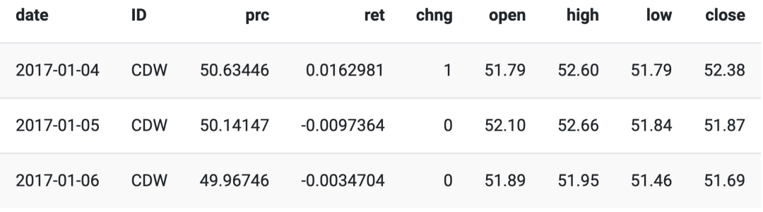
The first few observations of the data are as follows:
We can use the nest() function to put the data into a convenient nested table, which we can simply map over with map() and apply the rsample package’s rolling_origin() function, so that each of our assets will have its own rolling_origin() function applied to it without any overlap or mixing of asset classes, and we do this to create time series features for each cycle.
nested_df <- df %>%
  mutate(duplicate_ID = ID) %>%
  nest(-ID)
We will divide the time series data into multiple lists so that the analysis() list contains 100 observations in each list, and has a corresponding assessment() list with 1 observation. Typically, analysis() will become our training dataset, and assessment() will become our testing dataset, but here we use the rolling_origin() function to help create time series features.
rolled_df <- map(nested_df$data, ~ rolling_origin(.,
                                                  initial = 100,
                                                  assess = 1,
                                                  cumulative = FALSE,
                                                  skip = 0))
4
Time Series Functions
To create time series variables, we use the tsfeatures package, but there is also a feasts package here. For this model, we only need to select some functions of interest from the tsfeatures package.
functions <- c(
  "entropy",                   # Measures the "forecastability" of a series - low values = high sig-to-noise, large vals = difficult to forecast
  "stability",                 # means/variances are computed for all tiled windows - stability is the variance of the means
  "lumpiness",                 # Lumpiness is the variance of the variances
  "max_level_shift",           # Finds the largest mean shift between two consecutive windows (returns two values, size of shift and time index of shift)
  "max_var_shift",             # Finds the max variance shift between two consecutive windows (returns two values, size of shift and time index of shift)
  "max_kl_shift",              # Finds the largest shift in the Kulback-Leibler divergence between two consecutive windows (returns two values, size of shift and time index of shift)
  "crossing_points"            # Number of times a series crosses the mean line
)
We find it more interesting to stick with the map() function instead of function(SYMB). This function performs the following operations on each asset in our data:
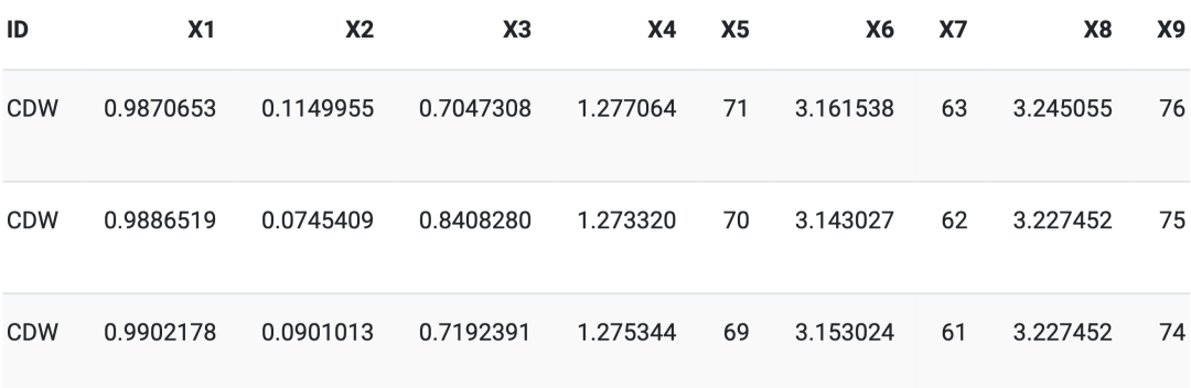
Using out-of-sample t+1 (assessment) data, bind these lists into a dataframe. Next, apply the functions string to call functions from the tsfeatures package, applying these functions to the sample analysis data (each data containing 100 observations), so we get a foldable set of observations that can be bound together. Finally, we use bind_cols() to bind the columns of the two datasets together. After that, we rename the chng variable and use ~str_c(“X”, seq_along(.)) to rename the time series feature variables to more dynamic variables, so we only need to add functions to the functions string without worrying about renaming variables separately to make the model work.
After completing this, we will use the rolling_origin() function again to create the machine learning dataset. The first rolling_origin() function is used to help fold time series data on a rolling basis by taking the previous 100 days of data and calculating the tsfeatures functions on it, which is similar to using the zoo package’s rollapply() function to calculate using rolling averages/standard deviations.
Next, we use the variables X_train and X_test to split the data into X variables and use Y_train and Y_test to separate the corresponding Y variables. The xgboost package requires a specific type of xgb.DMatrix(). This is what dtrain and dtest are doing.
Then, we set the XGBoost parameters and apply the XGBoost model. At this point, proper cross-validation should be performed, but since time series cross-validation is very tricky, there are no functions in R to help with this type of cross-validation. We will introduce the method to readers in a later article.
Once the model is trained, we start making predictions.
5
Model Application
The function for calculating all of this is as follows:
Prediction_Model <- function(SYMB){
  data <- bind_cols(
    map(rolled_df[[SYMB]]$splits, ~ assessment(.x)) %>%
      bind_rows(),
    map(rolled_df[[SYMB]]$splits, ~ analysis(.x)) %>%
      map(., ~tsfeatures(.x[["ret"]], functions)) %>%
      bind_rows()
  ) %>%
    rename(Y = chng) %>%
    rename_at(vars(-c(1:9)), ~str_c("X", seq_along(.)))

  ml_data <- data %>%
    as_tibble() %>%
    rolling_origin(
      initial    = 200,
      assess     = 1,
      cumulative = FALSE,
      skip       = 0)

  X_train <- map(
    ml_data$splits, ~ analysis(.x) %>%
      as_tibble(., .name_repair = "universal") %>%
      select(starts_with("X")) %>%
      as.matrix()
  )

  Y_train <- map(
    ml_data$splits, ~ analysis(.x) %>%
      as_tibble(., .name_repair = "universal") %>%
      select(starts_with("Y")) %>%
      as.matrix()
  )

  X_test <- map(
    ml_data$splits, ~ assessment(.x) %>%
      as_tibble(., .name_repair = "universal") %>%
      select(starts_with("X")) %>%
      as.matrix()
  )

  Y_test <- map(
    ml_data$splits, ~ assessment(.x) %>%
      as_tibble(., .name_repair = "universal") %>%
      select(starts_with("Y")) %>%
      as.matrix()
  )

  #############################################################

  dtrain <- map2(
    X_train, Y_train, ~ xgb.DMatrix(data = .x, label = .y, missing = "NaN")
  )

  dtest <- map(
    X_test, ~ xgb.DMatrix(data = .x, missing = "NaN")
  )

  # Parameters:
  watchlist <- list("train" = dtrain)
  params <- list("eta" = 0.1, "max_depth" = 5, "colsample_bytree" = 1, "min_child_weight" = 1, "subsample"= 1,
                 "objective"="binary:logistic", "gamma" = 1, "lambda" = 1, "alpha" = 0, "max_delta_step" = 0,
                 "colsample_bylevel" = 1, "eval_metric"= "auc",
                 "set.seed" = 176)

  # Train the XGBoost model
  xgb.model <- map(
    dtrain, ~ xgboost(params = params, data = .x, nrounds = 10, watchlist)
  )

  xgb.pred <- map2(
    .x = xgb.model,
    .y = dtest,
    .f = ~ predict(.x, newdata = .y, type = 'prob')
  )

  preds <- cbind(plyr::ldply(xgb.pred, data.frame),
                 plyr::ldply(Y_test, data.frame)) %>%
    setNames(c("pred_probs", "actual")) %>%
    bind_cols(plyr::ldply(map(ml_data$splits, ~assessment(.x)))) %>%
    rename(ID = duplicate_ID) %>%
    #select(pred_probs, actual, date, ID, prc, ret) %>%
    as_tibble()
  return(preds)
}
We can apply the above model to create time series features by training and testing each of our assets with the following:
Sys_t_start <- Sys.time()
Resultados <- lapply(seq(1:length(rolled_df)), Prediction_Model)
Sys_t_end <- Sys.time()
round(Sys_t_end - Sys_t_start, 2)
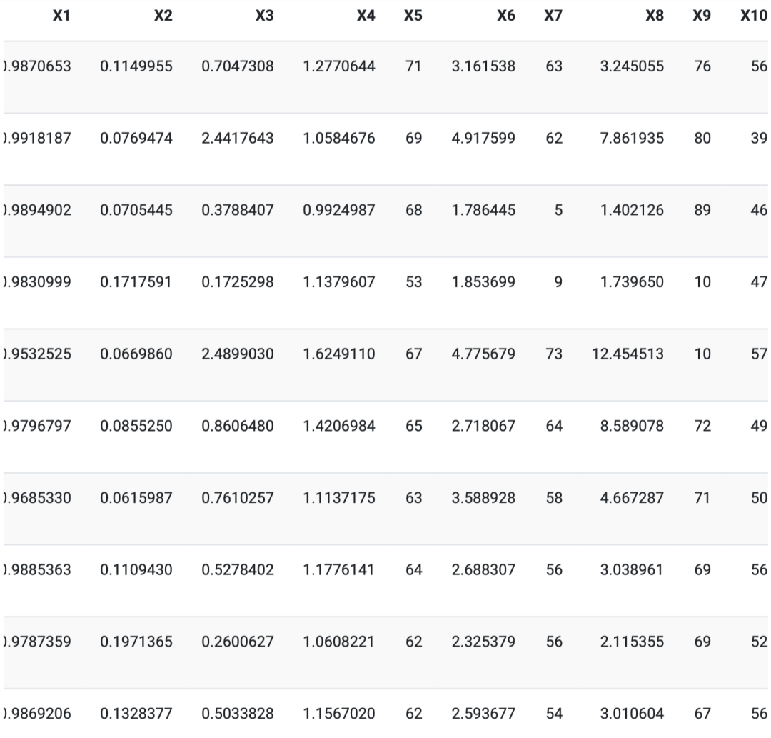
The Resultados output will give us a list that lists the length of the number of assets in our data. The first few observations of the first asset in the list are as follows:
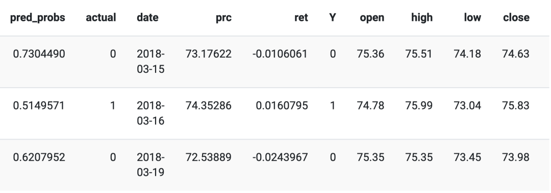
It includes the predicted probabilities from XGBoost, the actual observations, the result date (the date of the out-of-sample test data), the observed stock price, the calculated daily return (a copy of the observations), the OHLC data collected from Yahoo, and finally, we constructed time series features and then renamed them as
The goal of this strategy is to invest daily in the asset with the highest predicted probability of market appreciation. In other words, if the model predicts on day t that the price of GOOG will be above the previous closing price with a predicted probability of 0.78, and also predicts that AMZN will rise with a probability of 0.53, it is likely that we will invest in GOOG today. In other words, we only invest in the assets with the highest expected probability of market appreciation.
Therefore, we created a new data frame named top_assets, which essentially provides us with the highest predicted probabilities for all assets daily.
top_assets <- plyr::ldply(Resultados) %>%
  #select(pred_probs, actual, date, open, high, low, close, prc, ret) %>%
  group_by(date) %>%
  arrange(desc(pred_probs)) %>%
  dplyr::slice(1) %>%
  ungroup() %>%
  select(date, everything()) %>%
  rename(score = pred_probs) %>%
  select(-actual)
6
Strategy Evaluation
The first 10 days of strategy investment are as follows:
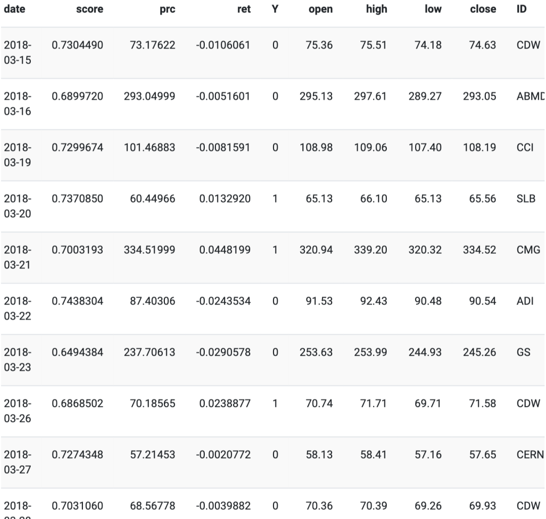
We can see that the score column is the probability of the asset with the highest predicted probability, that is, its price is higher than its previous closing price. The ID column provides us with the asset codes we invested in.
Next, we will analyze the strategy of selecting the best predicted winners based on the S&P 500 benchmark index and download the S&P 500 index.
top_assets <- xts(top_assets[,c(2:ncol(top_assets))], order.by = top_assets$date) # put top_assets into xts format

# Analyse strategy
getSymbols("SPY",
           from = start_date,
           to = end_date,
           src = "yahoo")
## [1] "SPY"
#detach("package:tsibble", unload = TRUE) # tsibble clashes with the base R index() function
SPY$ret_Rb <- Delt(SPY$SPY.Adjusted)
SPY <- SPY[index(SPY) >= min(index(top_assets))]

RaRb <- cbind(top_assets, SPY)
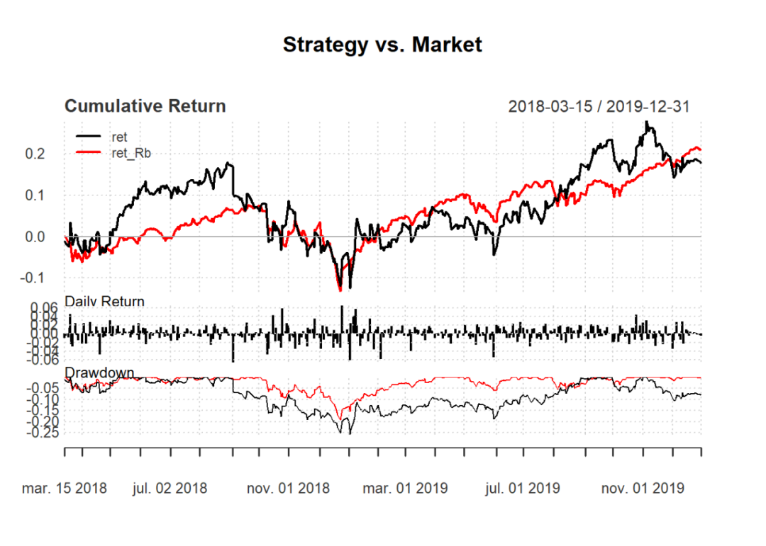
From here we can see the comparison of the strategy with the S&P 500 index. The model has not yet been extended to include short selling or constructing multi-asset portfolios of the top N assets.
Plotting the performance of the strategy:
charts.PerformanceSummary(RaRb[, c("ret", "ret_Rb")], geometric = FALSE, wealth.index = FALSE,
                          main = "Strategy vs. Market")
Relevant Metrics:
##                             ret ret_Rb
## Sterling ratio           0.1870 0.3879
## Calmar ratio             0.2551 0.5884
## Burke ratio              0.2251 0.5344
## Pain index               0.0955 0.0283
## Ulcer index              0.1189 0.0455
## Pain ratio               0.7337 4.0290
## Martin ratio             0.5891 2.5027
## daily downside risk      0.0111 0.0066
## Annualised downside risk 0.1768 0.1044
## Downside potential       0.0054 0.0029
## Omega                    1.0722 1.1601
## Sortino ratio            0.0351 0.0714
## Upside potential         0.0058 0.0034
## Upside potential ratio   0.7027 0.6124
## Omega-sharpe ratio       0.0722 0.1601
Backtesting Information:
## $ret
##         From     Trough         To   Depth Length To Trough Recovery
## 1 2018-08-31 2019-01-03 2019-09-16 -0.2746    261        85      176
## 2 2019-11-06 2019-12-03       <NA> -0.1300     39        19       NA
## 3 2019-10-01 2019-10-18 2019-10-29 -0.0810     21        14        7
## 4 2018-03-22 2018-04-20 2018-05-09 -0.0773     34        21       13
## 5 2018-08-10 2018-08-15 2018-08-20 -0.0474      7         4        3
##
## $ret_Rb
##         From     Trough         To   Depth Length To Trough Recovery
## 1 2018-09-21 2018-12-24 2019-04-12 -0.1935    140        65       75
## 2 2019-05-06 2019-06-03 2019-06-20 -0.0662     33        20       13
## 3 2018-03-15 2018-04-02 2018-06-04 -0.0610     56        12       44
## 4 2019-07-29 2019-08-05 2019-10-25 -0.0602     64         6       58
## 5 2018-06-13 2018-06-27 2018-07-09 -0.0300     18        11        7
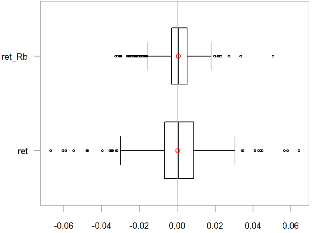
Comparing Returns
chart.Boxplot(RaRb[,c("ret", "ret_Rb")], main = "Returns")
Comparative Return Statistics:
table.Stats(RaRb[, c("ret", "ret_Rb")]) %>%
  t() %>%
  kable() %>%
  kable_styling(bootstrap_options = c("striped", "hover", "condensed", "responsive"))
    Observation  Asset Value  Minimum Requirement  Quartile 1  Median  Arithmetic Mean  Geometric Mean  Quartile 3  Maximum  SE Mean  LCL Mean (0.95)  UCL Mean (0.95)  Variance  Std Dev  Skewness  Kurtosis
Return  453 0 -0.0669 -0.0068 0.0006 0.0004 0.0003 0.0087 0.0642 0.0007 -0.0011 0.0018 0.0002 0.0156 -0.2542 2.8842
ret_Rb  453 0 -0.0324 -0.0030 0.0006 0.0005 0.0004 0.0054 0.0505 0.0004 -0.0004 0.0013 0.0001 0.0091 -0.2949 3.6264
Sharpe:
lapply(RaRb[, c("ret", "ret_Rb")], function(x){SharpeRatio(x)})
## $ret
##                                       ret
## StdDev Sharpe (Rf=0%, p=95%): 0.025027498
## VaR Sharpe (Rf=0%, p=95%):    0.015346462
## ES Sharpe (Rf=0%, p=95%):     0.009618405
##
## $ret_Rb
##                                   ret_Rb
## StdDev Sharpe (Rf=0%, p=95%): 0.05152014
## VaR Sharpe (Rf=0%, p=95%):    0.03218952
## ES Sharpe (Rf=0%, p=95%):     0.01913213
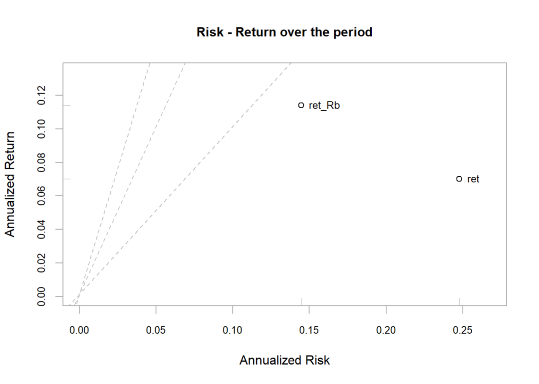
Plotting the risk-return scatter plot:
chart.RiskReturnScatter(RaRb[, c("ret", "ret_Rb")],
                        Rf=.03/252, scale = 252,
                        main = "Risk - Return over the period")
Plotting rolling returns, risks, and Sharpe performance:
charts.RollingPerformance(RaRb[, c("ret", "ret_Rb")],
                          Rf=.03/12,
                          colorset = c("red", rep("darkgray",5), "orange", "green"), lwd = 2)

Annualized Returns:
lapply(RaRb[, c("ret")],function(x){periodReturn(
  x, period = 'yearly', type = 'arithmetic')})
## $ret
##            yearly.returns
## 2018-12-31      -1.855083
## 2019-12-31      -1.475181
lapply(RaRb[, c("ret_Rb")],function(x){periodReturn(
  x, period = 'yearly', type = 'arithmetic')})
## $ret_Rb
##            yearly.returns
## 2018-12-31     -9.0376638
## 2019-12-31     -0.7226497
The WeChat public account for quantitative investment and machine learning is a mainstream self-media in the industry, vertical to fields such as Quant、Fintech、AI、ML and others. The public account has more than 180,000 followers from various circles including public funds, private equity, brokerage, futures, banks, insurance, and asset management. It publishes cutting-edge research results and the latest quantitative information daily.