

The XGBoost library provides an efficient implementation of gradient boosting, which can be configured to train a random forest ensemble. Random forests are simpler algorithms compared to gradient boosting. The XGBoost library allows for training random forest models in a way that reuses and takes advantage of the computational efficiency implemented in the library.In this tutorial, you will discover how to develop a random forest ensemble using the XGBoost library. By the end of this tutorial, you will know:
- XGBoost provides an efficient implementation of gradient boosting, which can be configured to train a random forest ensemble.
- How to train and evaluate random forest ensemble models for classification and regression using the XGBoost API.
- How to tune hyperparameters of the XGBoost random forest ensemble model.
Tutorial OverviewThis tutorial is divided into five sections. They are:
- Random Forests in XGBoost
- XGBoost API for Random Forests
- XGBoost Classification Random Forest
- XGBoost Regression Random Forest
- XGBoost Random Forest Hyperparameters
Random Forests in XGBoostXGBoost is an open-source library that provides an efficient implementation of the gradient boosting ensemble algorithm, abbreviated as Extreme Gradient Boosting or XGBoost. Thus, XGBoost refers to the project, the library, and the algorithm itself. Gradient boosting is the preferred algorithm for classification and regression predictive modeling projects because it often achieves the best performance. The problem with gradient boosting is that training the models is usually very slow, and large datasets exacerbate this issue. XGBoost addresses the speed issue by introducing many techniques that significantly accelerate the training of models and often lead to better overall model performance.You can learn more about XGBoost in this tutorial:
A Gentle Introduction to XGBoost for Applied Machine Learning
https://machinelearningmastery.com/gentle-introduction-xgboost-applied-machine-learning/
In addition to supporting gradient boosting, the core XGBoost algorithm can also be configured to support other types of tree ensemble algorithms, such as random forests. A random forest is a collection of decision tree algorithms. Each decision tree is fitted to a bootstrap sample of the training dataset. This is a sample of the training dataset where a given example (row) can be selected multiple times, known as a bootstrap sample. Importantly, a random subset of input variables (columns) is considered at each split point in the tree. This ensures that each tree added to the ensemble is skilled but differs in a random manner. The number of features considered at each split point is typically only a small subset. For example, in classification problems, a common heuristic is to select a number of features equal to the square root of the total number of features, so if the dataset has 20 input variables, it would be 4. You can learn more about the random forest ensemble algorithm in this tutorial:
How to Develop a Random Forest Ensemble in Python
https://machinelearningmastery.com/random-forest-ensemble-in-python/
The main advantage of training a random forest ensemble using the XGBoost library is speed. It is expected to be faster to use compared to other implementations, such as the native scikit-learn implementation. Now we know that XGBoost provides known performance relative to the baseline.XGBoost API for Random ForestsThe first step is to install the XGBoost library. I recommend using the following command from the command line with the pip package manager:
sudo pip install xgboost
Once installed, we can load the library and print the version using a Python script to confirm it is installed correctly.
# check xgboost version
import xgboost
# display version
print(xgboost.__version__)
Running the script will load the XGBoost library and print the version number of the library.Your version number should be the same or higher.
1.0.2
The XGBoost library provides two wrapper classes that allow the random forest implementation provided by the library to be used with the scikit-learn machine learning library.They are the XGBRFClassifier and XGBRFRegressor classes for classification and regression, respectively.
# define the model
model = XGBRFClassifier()
The number of trees used in the ensemble can be set via the “n_estimators” parameter, and this number is typically increased until no further performance improvement is observed in the model. Typically, hundreds or thousands of trees are used.
# define the model
model = XGBRFClassifier(n_estimators=100)
XGBoost does not support drawing bootstrap samples for each decision tree. This is a limitation of the library. Instead, you can specify a subsample of the training dataset as a percentage between 0.0 and 1.0 (100% of the rows in the training dataset) using the “subsample” parameter. It is recommended to use values of 0.8 or 0.9 to ensure the dataset is large enough to train a skilled model but diverse enough to introduce some variety into the ensemble.
# define the model
model = XGBRFClassifier(n_estimators=100, subsample=0.9)
When training the model, the number of features used at each split point can be specified via the “colsample_bynode” parameter, which takes a percentage of the number of columns in the dataset (from 0.0 to 1.0, representing 100% of input rows in the training dataset).If we have 20 input variables in the training dataset and the heuristic for classification problems is the square root of the number of features, we could set it to sqrt(20)/20, or approximately 4/20 or 0.2.
# define the model
model = XGBRFClassifier(n_estimators=100, subsample=0.9, colsample_bynode=0.2)
You can learn more about how to configure the XGBoost library for random forest ensembles here:
Random Forests in XGBoost
https://xgboost.readthedocs.io/en/latest/tutorials/rf.html
Now that we are familiar with how to define a random forest ensemble using the XGBoost API, let’s look at some actionable examples.XGBoost Classification Random ForestIn this section, we will explore developing XGBoost random forest ensembles for classification problems.First, we can create a synthetic binary classification problem with 1,000 examples and 20 input features using the <span>make_classification()</span> function.The complete example is listed below.
# test classification dataset
from sklearn.datasets import make_classification
# define dataset
X, y = make_classification(n_samples=1000, n_features=20, n_informative=15, n_redundant=5, random_state=7)
# summarize the dataset
print(X.shape, y.shape)
Running the example will create the dataset and summarize the shape of the input and output components.
(1000, 20) (1000,)
Next, we can evaluate the XGBoost random forest algorithm on this dataset.We will evaluate the model using repeated stratified k-fold cross-validation (with 3 repeats and 10 folds). We will report the mean and standard deviation of the model accuracy across all repeats and folds.
# evaluate xgboost random forest algorithm for classification
from numpy import mean
from numpy import std
from sklearn.datasets import make_classification
from sklearn.model_selection import cross_val_score
from sklearn.model_selection import RepeatedStratifiedKFold
from xgboost import XGBRFClassifier
# define dataset
X, y = make_classification(n_samples=1000, n_features=20, n_informative=15, n_redundant=5, random_state=7)
# define the model
model = XGBRFClassifier(n_estimators=100, subsample=0.9, colsample_bynode=0.2)
# define the model evaluation procedure
cv = RepeatedStratifiedKFold(n_splits=10, n_repeats=3, random_state=1)
# evaluate the model and collect the scores
n_scores = cross_val_score(model, X, y, scoring='accuracy', cv=cv, n_jobs=-1)
# report performance
print('Mean Accuracy: %.3f (%.3f)' % (mean(n_scores), std(n_scores)))
Running the example will report the mean and standard deviation accuracy of the model.Note: Your results may vary due to the randomness of the algorithm or evaluation procedure, or differences in numerical precision. Consider running the example several times and comparing the average results.In this case, we can see that the XGBoost random forest ensemble achieved approximately 89.1% classification accuracy.
Mean Accuracy: 0.891 (0.036)
We can also use the XGBoost random forest model as the final model and make classification predictions.First, fit the XGBoost random forest ensemble on all available data, then the <span>predict()</span> function can be called to make predictions on new data.The following example demonstrates this in our binary classification dataset.
# make predictions using xgboost random forest for classification
from numpy import asarray
from sklearn.datasets import make_classification
from xgboost import XGBRFClassifier
# define dataset
X, y = make_classification(n_samples=1000, n_features=20, n_informative=15, n_redundant=5, random_state=7)
# define the model
model = XGBRFClassifier(n_estimators=100, subsample=0.9, colsample_bynode=0.2)
# fit the model on the whole dataset
model.fit(X, y)
# define a row of data
row = [0.2929949,-4.21223056,-1.288332,-2.17849815,-0.64527665,2.58097719,0.28422388,-7.1827928,-1.91211104,2.73729512,0.81395695,3.96973717,-2.66939799,3.34692332,4.19791821,0.99990998,-0.30201875,-4.43170633,-2.82646737,0.44916808]
row = asarray([row])
# make a prediction
yhat = model.predict(row)
# summarize the prediction
print('Predicted Class: %d' % yhat[0])
Running the example will fit the XGBoost random forest ensemble model on the entire dataset and then use it to make predictions on a new row of data, just as we would use the model in an application.
Predicted Class: 1
Now that we are familiar with how to use random forests for classification, let’s look at the API for regression.XGBoost Regression Random ForestIn this section, we will explore developing XGBoost random forest ensembles for regression problems. First, we can create a synthetic regression problem with 1,000 examples and 20 input features using the <span>make_regression()</span> function. The complete example is listed below.
# test regression dataset
from sklearn.datasets import make_regression
# define dataset
X, y = make_regression(n_samples=1000, n_features=20, n_informative=15, noise=0.1, random_state=7)
# summarize the dataset
print(X.shape, y.shape)
Running the example will create the dataset and summarize the shape of the input and output components.
(1000, 20) (1000,)
Next, we can evaluate the XGBoost random forest ensemble on this dataset.As we did in the previous section, we will use repeated k-fold cross-validation (with three repeats and 10 folds) to evaluate the model.We will report the mean absolute error (MAE) of the model across all repeats and folds. The scikit-learn library makes MAE negative, maximizing instead of minimizing it. This means that a larger negative MAE is better, and an ideal model has an MAE of 0.The complete example is listed below.
# evaluate xgboost random forest ensemble for regression
from numpy import mean
from numpy import std
from sklearn.datasets import make_regression
from sklearn.model_selection import cross_val_score
from sklearn.model_selection import RepeatedKFold
from xgboost import XGBRFRegressor
# define dataset
X, y = make_regression(n_samples=1000, n_features=20, n_informative=15, noise=0.1, random_state=7)
# define the model
model = XGBRFRegressor(n_estimators=100, subsample=0.9, colsample_bynode=0.2)
# define the model evaluation procedure
cv = RepeatedKFold(n_splits=10, n_repeats=3, random_state=1)
# evaluate the model and collect the scores
n_scores = cross_val_score(model, X, y, scoring='neg_mean_absolute_error', cv=cv, n_jobs=-1)
# report performance
print('MAE: %.3f (%.3f)' % (mean(n_scores), std(n_scores)))
Running the example will report the mean and standard deviation MAE of the model.Note: Your results may vary due to the randomness of the algorithm or evaluation procedure, or differences in numerical precision. Consider running the example several times and comparing the average results.In this case, we can see that the random forest ensemble with default hyperparameters achieved an MAE of around 108.
MAE: -108.290 (5.647)
We can also use the XGBoost random forest ensemble as the final model and make regression predictions.First, fit the random forest ensemble on all available data, then the <span>predict()</span> function can be called to make predictions on new data.The following example demonstrates this in our regression dataset.
# gradient xgboost random forest for making predictions for regression
from numpy import asarray
from sklearn.datasets import make_regression
from xgboost import XGBRFRegressor
# define dataset
X, y = make_regression(n_samples=1000, n_features=20, n_informative=15, noise=0.1, random_state=7)
# define the model
model = XGBRFRegressor(n_estimators=100, subsample=0.9, colsample_bynode=0.2)
# fit the model on the whole dataset
model.fit(X, y)
# define a single row of data
row = [0.20543991,-0.97049844,-0.81403429,-0.23842689,-0.60704084,-0.48541492,0.53113006,2.01834338,-0.90745243,-1.85859731,-1.02334791,-0.6877744,0.60984819,-0.70630121,-1.29161497,1.32385441,1.42150747,1.26567231,2.56569098,-0.11154792]
row = asarray([row])
# make a prediction
yhat = model.predict(row)
# summarize the prediction
print('Prediction: %d' % yhat[0])
Running the example will fit the XGBoost random forest ensemble model on the entire dataset and then use it to make predictions on a new row of data, just as we would use the model in an application.
Prediction: 17
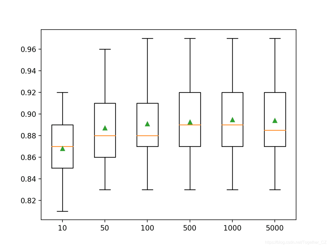
Now that we are familiar with how to develop and evaluate XGBoost random forest ensembles, let’s look at configuring the model.XGBoost Random Forest HyperparametersIn this section, we will take a closer look at some hyperparameters that you should consider tuning for random forest ensembles and their impact on model performance.Exploring the Number of TreesThe number of trees is another key hyperparameter to configure for XGBoost random forests. Generally, the number of trees is increased until the model performance stabilizes. Intuition might suggest that more trees would lead to overfitting, but this is not the case. Given the randomness of the learning algorithm, both bagging and random forest algorithms seem less prone to overfitting the training dataset. The number of trees can be set via the “n_estimators” parameter, which defaults to 100. The example below explores the effect of the number of trees with values ranging from 10 to 1,000.
# explore xgboost random forest number of trees effect on performance
from numpy import mean
from numpy import std
from sklearn.datasets import make_classification
from sklearn.model_selection import cross_val_score
from sklearn.model_selection import RepeatedStratifiedKFold
from xgboost import XGBRFClassifier
from matplotlib import pyplot

# get the dataset
def get_dataset():
    X, y = make_classification(n_samples=1000, n_features=20, n_informative=15, n_redundant=5, random_state=7)
    return X, y

# get a list of models to evaluate
def get_models():
    models = dict()
    # define the number of trees to consider
    n_trees = [10, 50, 100, 500, 1000, 5000]
    for v in n_trees:
        models[str(v)] = XGBRFClassifier(n_estimators=v, subsample=0.9, colsample_bynode=0.2)
    return models

# evaluate a given model using cross-validation
def evaluate_model(model, X, y):
    # define the model evaluation procedure
    cv = RepeatedStratifiedKFold(n_splits=10, n_repeats=3, random_state=1)
    # evaluate the model
    scores = cross_val_score(model, X, y, scoring='accuracy', cv=cv, n_jobs=-1)
    return scores

# define dataset
X, y = get_dataset()
# get the models to evaluate
models = get_models()
# evaluate the models and store results
results, names = list(), list()
for name, model in models.items():
    # evaluate the model and collect the results
    scores = evaluate_model(model, X, y)
    # store the results
    results.append(scores)
    names.append(name)
    # summarize performance along the way
    print('>%s %.3f (%.3f)' % (name, mean(scores), std(scores)))
# plot model performance for comparison
pyplot.boxplot(results, labels=names, showmeans=True)
pyplot.show()
Running the example will report the mean accuracy for each configured number of trees.Note: Your results may vary due to the randomness of the algorithm or evaluation procedure, or differences in numerical precision. Consider running the example several times and comparing the average results.In this case, we can see that performance rises and stabilizes after about 500 trees. The average accuracy scores fluctuate at 500, 1,000, and 5,000 trees, which may be statistical noise.
>10 0.868 (0.030)
>50 0.887 (0.034)
>100 0.891 (0.036)
>500 0.893 (0.033)
>1000 0.895 (0.035)
>5000 0.894 (0.036)
Create a box plot to assign accuracy scores for each configured number of trees.
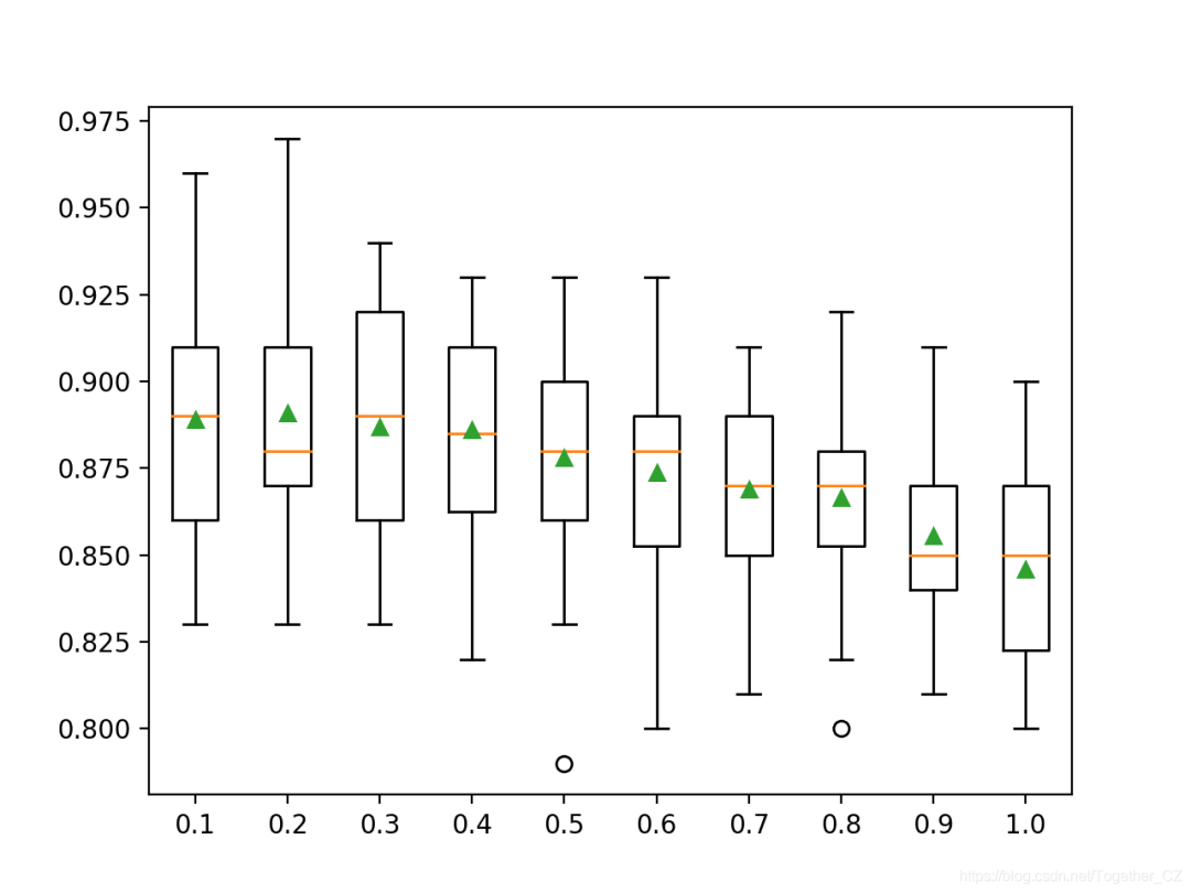
Exploring the Number of FeaturesThe number of features randomly sampled at each split point may be the most important factor to configure for random forests. This is set via the “colsample_bynode” parameter, which is a percentage of the number of input features (from 0 to 1). The example below explores the effect of the number of features randomly selected at each split point on model accuracy. We will try values from 0.0 to 1.0 in increments of 0.1, although we expect that values below 0.2 or 0.3 will yield good or optimal performance, as this translates to the square root of the number of input features, which is a common heuristic.
# explore xgboost random forest number of features effect on performance
from numpy import mean
from numpy import std
from numpy import arange
from sklearn.datasets import make_classification
from sklearn.model_selection import cross_val_score
from sklearn.model_selection import RepeatedStratifiedKFold
from xgboost import XGBRFClassifier
from matplotlib import pyplot

# get the dataset
def get_dataset():
    X, y = make_classification(n_samples=1000, n_features=20, n_informative=15, n_redundant=5, random_state=7)
    return X, y

# get a list of models to evaluate
def get_models():
    models = dict()
    for v in arange(0.1, 1.1, 0.1):
        key = '%.1f' % v
        models[key] = XGBRFClassifier(n_estimators=100, subsample=0.9, colsample_bynode=v)
    return models

# evaluate a given model using cross-validation
def evaluate_model(model, X, y):
    # define the model evaluation procedure
    cv = RepeatedStratifiedKFold(n_splits=10, n_repeats=3, random_state=1)
    # evaluate the model
    scores = cross_val_score(model, X, y, scoring='accuracy', cv=cv, n_jobs=-1)
    return scores

# define dataset
X, y = get_dataset()
# get the models to evaluate
models = get_models()
# evaluate the models and store results
results, names = list(), list()
for name, model in models.items():
    # evaluate the model and collect the results
    scores = evaluate_model(model, X, y)
    # store the results
    results.append(scores)
    names.append(name)
    # summarize performance along the way
    print('>%s %.3f (%.3f)' % (name, mean(scores), std(scores)))
# plot model performance for comparison
pyplot.boxplot(results, labels=names, showmeans=True)
pyplot.show()
Running the example will report the mean accuracy for each feature set size.Note: Your results may vary due to the randomness of the algorithm or evaluation procedure, or differences in numerical precision. Consider running the example several times and comparing the average results.In this case, as the ensemble members use more input features, we can see an overall trend of decreasing average model performance.The results suggest that a recommended value of 0.2 would be a good choice in this case.
>0.1 0.889 (0.032)
>0.2 0.891 (0.036)
>0.3 0.887 (0.032)
>0.4 0.886 (0.030)
>0.5 0.878 (0.033)
>0.6 0.874 (0.031)
>0.7 0.869 (0.027)
>0.8 0.867 (0.027)
>0.9 0.856 (0.023)
>1.0 0.846 (0.027)
Create a box plot to assign accuracy scores for each feature set size.We can see the trend of performance decreasing with the number of features considered in the decision trees.
Author: Yishui Hancheng, CSDN Blog Expert, personal research areas: Machine Learning, Deep Learning, NLP, CV
Blog: http://yishuihancheng.blog.csdn.net
Support the Author

More Reading
Time Series Forecasting with XGBoost
Master Python Random Hill Climbing Algorithm in 5 Minutes
Fully Understand Association Rule Mining Algorithm in 5 Minutes
Special Recommendation


Click below to read the original text and join the community members