

XGBoost is an effective implementation for gradient classification and regression problems.It is fast and efficient, performing excellently in various predictive modeling tasks and is widely favored among winners of data science competitions (e.g., Kaggle winners), even if it is not the best.XGBoost can also be used for time series forecasting, although it requires converting the time series dataset into a supervised learning problem first. It also requires a specialized technique for model evaluation called forward validation, as using k-fold cross-validation can lead to optimistic results.In this tutorial, you will learn how to develop an XGBoost model for time series forecasting. By the end of this tutorial, you will know:1. XGBoost is an implementation of the gradient boosting ensemble algorithm for classification and regression.2. Time series datasets can be converted into supervised learning using a sliding window representation.3. How to fit, evaluate, and make predictions with the XGBoost model for time series forecasting.Tutorial OverviewThis tutorial is divided into three parts:1. XGBoost Ensemble2. Time Series Data Preparation3. XGBoost for Time Series ForecastingXGBoost EnsembleXGBoost stands for Extreme Gradient Boosting, an effective implementation of the stochastic gradient boosting machine learning algorithm. The stochastic gradient boosting algorithm (also known as gradient boosted trees or tree boosting) is a powerful machine learning technique that performs excellently on various challenging machine learning problems, often achieving the best results.It is a collection of decision tree algorithms where new trees fix the errors of those trees already in the model. Trees are added until no further improvements can be made to the model. XGBoost provides an efficient implementation of the stochastic gradient boosting algorithm and offers a set of model hyperparameters designed to provide control over the model training process.XGBoost is designed for classification and regression of tabular datasets, although it can be used for time series forecasting.First, you must install the XGBoost library. You can install it using pip as follows:
sudo pip install xgboost
Once installed, you can confirm it has been successfully installed and that you are using a modern version by running the following code:
# xgboost
import xgboost
print("xgboost", xgboost.__version__)
When you run the code, you should see the following version number or higher.
xgboost 1.0.1
Although the XGBoost library has its own Python API, we can use the XGBRegressor wrapper class to integrate the XGBoost model with the scikit-learn API.An instance of the model can be instantiated just like any other scikit-learn class used for model evaluation. For example:
# define model
model = XGBRegressor()
Now that we are familiar with XGBoost, let’s see how to prepare a time series dataset for supervised learning.Time Series Data PreparationTime series data can be expressed as supervised learning. Given a sequence of numbers in a time series dataset, we can reorganize the data to resemble a supervised learning problem. We can do this by using previous time steps as input variables and the next time step as the output variable. Let’s illustrate this with an example. Suppose we have a time series as follows:
time, measure
1, 100
2, 110
3, 108
4, 115
5, 120
By predicting the value of the next time step using the value from the previous time step, we can reorganize this time series dataset into a supervised learning problem. When reorganizing the time series dataset in this way, the data will look like this:
X, y
?, 100
100, 110
110, 108
108, 115
115, 120
120, ?
Note that the time column has been removed, and certain data rows are not available for training the model, such as the first and last ones.This representation is called a sliding window, as the window of input and expected output moves forward over time, creating new “samples” for the supervised learning model.For more information on preparing time series forecasting data with the sliding window method.Given the desired lengths of input and output sequences, we can use the shift() function in Pandas to automatically create a new framework for the time series problem.This will be a useful tool as it will allow us to explore different frameworks of the time series problem using machine learning algorithms to see what might lead to better-performing models.The following function transforms a time series as a NumPy array with one or more columns into a supervised learning problem with a specified number of inputs and outputs.
# transform a time series dataset into a supervised learning dataset
def series_to_supervised(data, n_in=1, n_out=1, dropnan=True):
 n_vars = 1 if type(data) is list else data.shape[1]
 df = DataFrame(data)
 cols = list()
 # input sequence (t-n, ... t-1)
 for i in range(n_in, 0, -1):
  cols.append(df.shift(i))
 # forecast sequence (t, t+1, ... t+n)
 for i in range(0, n_out):
  cols.append(df.shift(-i))
 # put it all together
 agg = concat(cols, axis=1)
 # drop rows with NaN values
 if dropnan:
  agg.dropna(inplace=True)
 return agg.values
We can use this function to prepare the time series dataset for XGBoost.Once the dataset is ready, we must be careful about how we use it to fit and evaluate the model.For example, fitting the model on future data and predicting past values is invalid. The model must be trained on past data and predict future values. This means that methods that randomize the dataset during evaluation, such as k-fold cross-validation, cannot be used. Instead, we must use a technique called forward validation. In forward validation, we first train by selecting a cutoff point (e.g., using all data except the last 12 months for training and the most recent 12 months for testing).If we are interested in one-step predictions, such as one month ahead, we can evaluate the model by training on the training dataset and predicting the first step of the test dataset. Then we can add the actual observations from the test set to the training dataset, refit the model, and let the model predict the second step in the test dataset. Repeating this process for the entire test dataset will provide one-step predictions for the entire test dataset, from which error metrics can be calculated to assess the model’s skill.The following function performs forward validation. It uses the entire supervised version of the time series dataset along with the number of rows used as the test set as parameters. It then steps through the test set, calling the xgboost_forecast() function for one-step predictions. It calculates error metrics and returns details for analysis.
# walk-forward validation for univariate data
def walk_forward_validation(data, n_test):
 predictions = list()
 # split dataset
 train, test = train_test_split(data, n_test)
 # seed history with training dataset
 history = [x for x in train]
 # step over each time-step in the test set
 for i in range(len(test)):
  # split test row into input and output columns
  testX, testy = test[i, :-1], test[i, -1]
  # fit model on history and make a prediction
  yhat = xgboost_forecast(history, testX)
  # store forecast in list of predictions
  predictions.append(yhat)
  # add actual observation to history for the next loop
  history.append(test[i])
  # summarize progress
  print('>expected=%.1f, predicted=%.1f' % (testy, yhat))
 # estimate prediction error
 error = mean_absolute_error(test[:, -1], predictions)
 return error, test[:, 1], predictions
Calling the train_test_split() function can split the dataset into training and testing sets. We can define this function below.
# split a univariate dataset into train/test sets
def train_test_split(data, n_test):
 return data[:-n_test, :], data[-n_test:, :]
We can use the XGBRegressor class for one-step predictions. The following xgboost_forecast() function implements this by fitting the model and making a one-step prediction using the training dataset and the test input row as input.
# fit an xgboost model and make a one step prediction
def xgboost_forecast(train, testX):
 # transform list into array
 train = asarray(train)
 # split into input and output columns
 trainX, trainy = train[:, :-1], train[:, -1]
 # fit model
 model = XGBRegressor(objective='reg:squarederror', n_estimators=1000)
 model.fit(trainX, trainy)
 # make a one-step prediction
 yhat = model.predict([testX])
 return yhat[0]
Now that we know how to prepare time series data for forecasting and evaluate the XGBoost model, we can look at using XGBoost on real datasets.XGBoost for Time Series ForecastingIn this section, we will explore how to use XGBoost for time series forecasting. We will use a standard univariate time series dataset to make one-step predictions with this model. You can use the code in this section as a starting point for your own projects and easily adjust it for multivariate inputs, multivariate predictions, and multi-step forecasts. We will use the daily female birth dataset, which contains the number of births per month over a three-year period.You can download the dataset from here and place it in the current working directory with the filename “daily-total-female-births.csv”.Dataset (daily female births total.csv):
https://raw.githubusercontent.com/jbrownlee/Datasets/master/daily-total-female-births.csv
Description (daily female births total):
https://raw.githubusercontent.com/jbrownlee/Datasets/master/daily-total-female-births.names
The first few rows of the dataset are as follows:
"Date","Births"
"1959-01-01",35
"1959-01-02",32
"1959-01-03",30
"1959-01-04",31
"1959-01-05",44
...
First, let’s load and plot the dataset. Below is a complete example.
# load and plot the time series dataset
from pandas import read_csv
from matplotlib import pyplot
# load dataset
series = read_csv('daily-total-female-births.csv', header=0, index_col=0)
values = series.values
# plot dataset
pyplot.plot(values)
pyplot.show()
Running the example will create a line plot of the dataset. We can see that there is no apparent trend or seasonality.
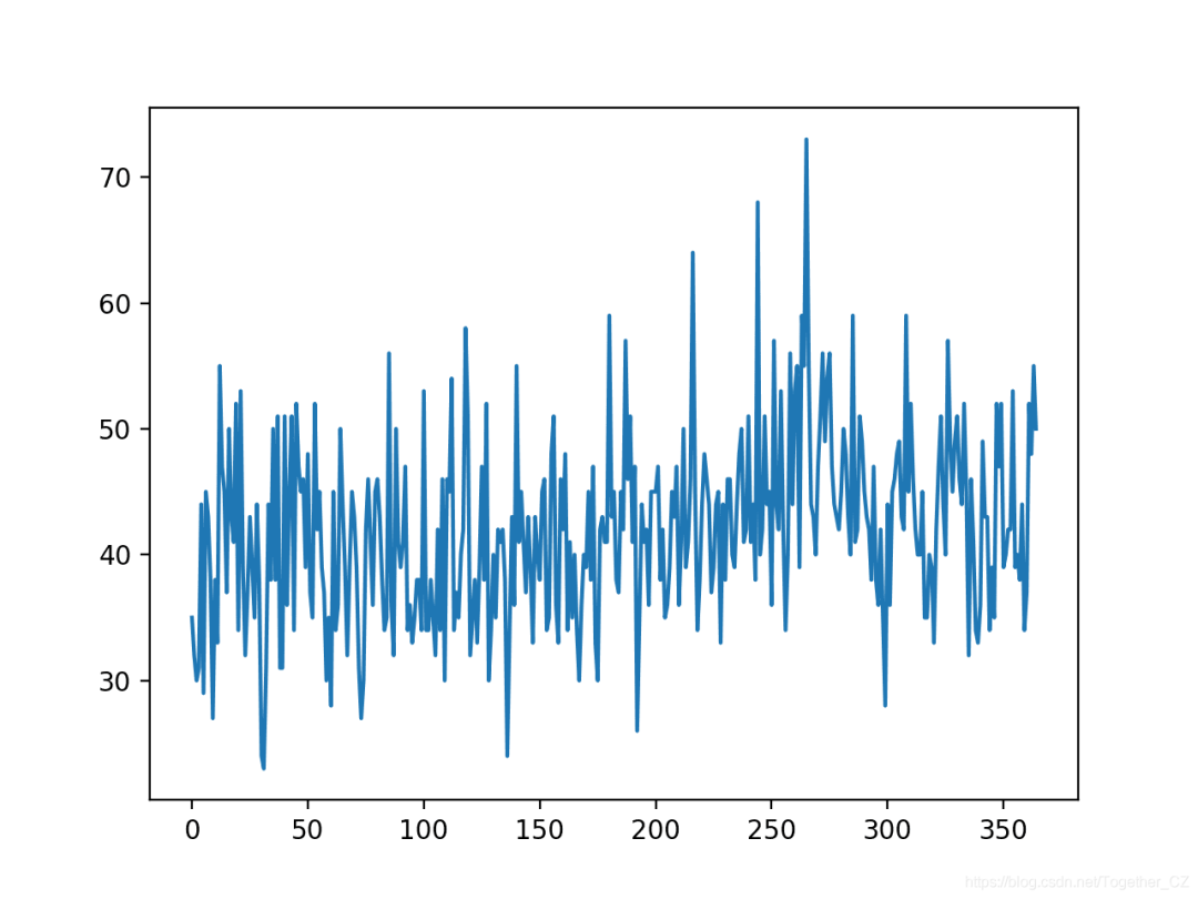
When forecasting the most recent 12 months, a persistence model can achieve an MAE of about 6.7 births. This provides a performance baseline above which a model can be considered skilled.Next, when making one-step predictions on the past 12 months of data, we can evaluate the XGBoost model on the dataset.We will use only the first 6 time steps as input to the model and the default model hyperparameters, except we will change the loss to ‘reg:squarederror’ (to avoid warning messages) and use 1,000 trees in the ensemble (to avoid underfitting).Below is a complete example.
# forecast monthly births with xgboost
from numpy import asarray
from pandas import read_csv
from pandas import DataFrame
from pandas import concat
from sklearn.metrics import mean_absolute_error
from xgboost import XGBRegressor
from matplotlib import pyplot

# transform a time series dataset into a supervised learning dataset
def series_to_supervised(data, n_in=1, n_out=1, dropnan=True):
 n_vars = 1 if type(data) is list else data.shape[1]
 df = DataFrame(data)
 cols = list()
 # input sequence (t-n, ... t-1)
 for i in range(n_in, 0, -1):
  cols.append(df.shift(i))
 # forecast sequence (t, t+1, ... t+n)
 for i in range(0, n_out):
  cols.append(df.shift(-i))
 # put it all together
 agg = concat(cols, axis=1)
 # drop rows with NaN values
 if dropnan:
  agg.dropna(inplace=True)
 return agg.values

# split a univariate dataset into train/test sets
def train_test_split(data, n_test):
 return data[:-n_test, :], data[-n_test:, :]

# fit an xgboost model and make a one step prediction
def xgboost_forecast(train, testX):
 # transform list into array
 train = asarray(train)
 # split into input and output columns
 trainX, trainy = train[:, :-1], train[:, -1]
 # fit model
 model = XGBRegressor(objective='reg:squarederror', n_estimators=1000)
 model.fit(trainX, trainy)
 # make a one-step prediction
 yhat = model.predict(asarray([testX]))
 return yhat[0]

# walk-forward validation for univariate data
def walk_forward_validation(data, n_test):
 predictions = list()
 # split dataset
 train, test = train_test_split(data, n_test)
 # seed history with training dataset
 history = [x for x in train]
 # step over each time-step in the test set
 for i in range(len(test)):
  # split test row into input and output columns
  testX, testy = test[i, :-1], test[i, -1]
  # fit model on history and make a prediction
  yhat = xgboost_forecast(history, testX)
  # store forecast in list of predictions
  predictions.append(yhat)
  # add actual observation to history for the next loop
  history.append(test[i])
  # summarize progress
  print('>expected=%.1f, predicted=%.1f' % (testy, yhat))
 # estimate prediction error
 error = mean_absolute_error(test[:, -1], predictions)
 return error, test[:, -1], predictions

# load the dataset
series = read_csv('daily-total-female-births.csv', header=0, index_col=0)
values = series.values
# transform the time series data into supervised learning
data = series_to_supervised(values, n_in=6)
# evaluate
mae, y, yhat = walk_forward_validation(data, 12)
print('MAE: %.3f' % mae)
# plot expected vs predicted
pyplot.plot(y, label='Expected')
pyplot.plot(yhat, label='Predicted')
pyplot.legend()
pyplot.show()
Running the example will report the expected and predicted values for each step in the test set, then report the MAE for all predictions.Note: Due to the randomness of the algorithm or evaluation procedure, or differences in numerical precision, your results may vary. Consider running the example several times and comparing the average results.We can see that the model performs better than the persistence model, with an MAE of about 5.9 compared to 6.7.
>expected=42.0, predicted=44.5
>expected=53.0, predicted=42.5
>expected=39.0, predicted=40.3
>expected=40.0, predicted=32.5
>expected=38.0, predicted=41.1
>expected=44.0, predicted=45.3
>expected=34.0, predicted=40.2
>expected=37.0, predicted=35.0
>expected=52.0, predicted=32.5
>expected=48.0, predicted=41.4
>expected=55.0, predicted=46.6
>expected=50.0, predicted=47.2
MAE: 5.957
Create a line plot comparing the series of expected and predicted values for the last 12 months of the dataset. This gives a geometric interpretation of how well the model performed on the test set.Figure 2Once the final configuration of the XGBoost model is chosen, the model can be finalized and used for predictions on new data. This is called out-of-sample forecasting, such as predicting beyond the training dataset. This is the same as making predictions during model evaluation: because we always want to evaluate the model using the same process that we expect to use when making predictions on new data. The following example demonstrates the process of fitting the final XGBoost model on all available data and making a one-step prediction at the end of the dataset.
# finalize model and make a prediction for monthly births with xgboost
from numpy import asarray
from pandas import read_csv
from pandas import DataFrame
from pandas import concat
from xgboost import XGBRegressor

# transform a time series dataset into a supervised learning dataset
def series_to_supervised(data, n_in=1, n_out=1, dropnan=True):
 n_vars = 1 if type(data) is list else data.shape[1]
 df = DataFrame(data)
 cols = list()
 # input sequence (t-n, ... t-1)
 for i in range(n_in, 0, -1):
  cols.append(df.shift(i))
 # forecast sequence (t, t+1, ... t+n)
 for i in range(0, n_out):
  cols.append(df.shift(-i))
 # put it all together
 agg = concat(cols, axis=1)
 # drop rows with NaN values
 if dropnan:
  agg.dropna(inplace=True)
 return agg.values

# load the dataset
series = read_csv('daily-total-female-births.csv', header=0, index_col=0)
values = series.values
# transform the time series data into supervised learning
train = series_to_supervised(values, n_in=6)
# split into input and output columns
trainX, trainy = train[:, :-1], train[:, -1]
# fit model
model = XGBRegressor(objective='reg:squarederror', n_estimators=1000)
model.fit(trainX, trainy)
# construct an input for a new prediction
row = values[-6:].flatten()
# make a one-step prediction
yhat = model.predict(asarray([row]))
print('Input: %s, Predicted: %.3f' % (row, yhat[0]))
Running the example will fit the XGBoost model on all available data. Using the known data from the last 6 months, it prepares a new input row and predicts the next month after the end of the dataset.
Input: [34 37 52 48 55 50], Predicted: 42.708
Author: Yishui Hancheng, CSDN Blog Expert, personal research focus: Machine Learning, Deep Learning, NLP, CV
Blog: http://yishuihancheng.blog.csdn.net
Support the Author

More Reading
Implement Simple Genetic Algorithm in Python from Scratch
Master Python Random Hill Climbing Algorithm in 5 Minutes
Completely Understand Association Rule Mining Algorithm in 5 Minutes
Special Recommendations


Click below to read the original text and join the community membership