Author on Zhihu | master苏
Link | https://zhuanlan.zhihu.com/p/139617364
This article introduces the visualization of the structure of LSTM models.
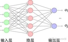
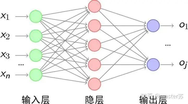
Traditional BP Networks and CNN Networks
BP networks and CNN networks do not have a time dimension, and they are quite similar to traditional machine learning algorithms in terms of understanding. When CNN processes a color image with three channels, it can also be understood as stacking multiple layers. The three-dimensional matrix of the image can be viewed as spatial slices, and one can simply follow the diagram and stack layers when writing code. The following image shows a typical BP network and a CNN network.
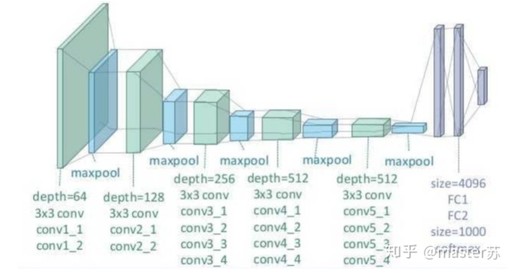
CNN Network
The hidden layers, convolutional layers, pooling layers, and fully connected layers in the diagram all exist in reality, stacked layer by layer, which is easy to understand spatially. Therefore, when writing code, one basically looks at the diagram to write code. For instance, using Keras, it would look like this:
<span># Example code, not practically significant</span><span>model = Sequential()</span><span>model.add(Conv2D(32, (3, 3), activation='relu')) # Add convolutional layer</span><span>model.add(MaxPooling2D(pool_size=(2, 2))) # Add pooling layer</span><span>model.add(Dropout(0.25)) # Add dropout layer</span><span>model.add(Conv2D(32, (3, 3), activation='relu')) # Add convolutional layer</span><span>model.add(MaxPooling2D(pool_size=(2, 2))) # Add pooling layer</span><span>model.add(Dropout(0.25)) # Add dropout layer</span><span>.... # Add other convolution operations</span><span>model.add(Flatten()) # Flatten 3D array to 2D array</span><span>model.add(Dense(256, activation='relu')) # Add regular fully connected layer</span><span>model.add(Dropout(0.5))model.add(Dense(10, activation='softmax'))</span><span>.... # Train the network</span>LSTM Networks
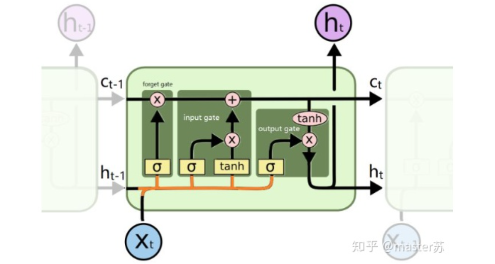
When we search for LSTM structures online, the most common image we see is the one below:

RNN Network
This is the classic structure diagram of RNN (Recurrent Neural Network), and LSTM is merely an improvement on the hidden layer node A, with the overall structure remaining unchanged. Thus, this article also discusses the visualization of this structure.
The middle A node represents the hidden layer, and the left side indicates an LSTM network with only one hidden layer. The so-called LSTM recurrent neural network utilizes cycles on the time axis, which is expanded on the time axis to yield the right diagram.
Looking at the left diagram, many students mistakenly think that LSTM has a single input and output, with only one hidden neuron in the network structure. However, viewing the right diagram, they believe that LSTM has multiple inputs and outputs, with several hidden neurons in the network structure; the number of A nodes represents the number of hidden layer nodes.
What the heck? It’s hard to wrap my head around this. This reflects the traditional network and spatial structure thinking.
In actuality, in the right diagram, Xt represents the sequence, and the subscript t is the time axis. Therefore, the number of A indicates the length of the time axis, representing the state (Ht) of the same neuron at different times, not the number of hidden layer neurons.
We know that the LSTM network uses information from the previous moment along with the current input information to jointly train during training.
For example: On the first day, I got sick (initial state H0), then took medicine (using input information X1 to train the network), on the second day I improved but was not completely well (H1), took medicine again (X2), and my condition improved (H2), repeating this cycle until I recovered. Thus, the input Xt is taking medicine, the time axis T is the number of days of medication, and the hidden layer state is the condition. Therefore, I am still me, just in different states.
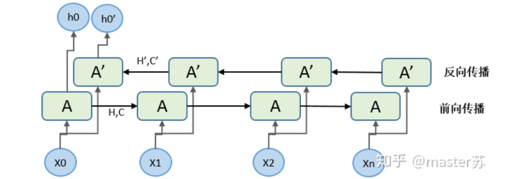
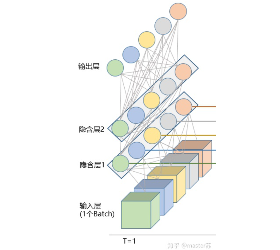
In reality, the LSTM network looks like this:
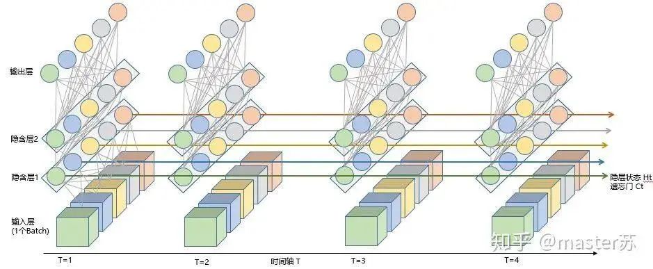
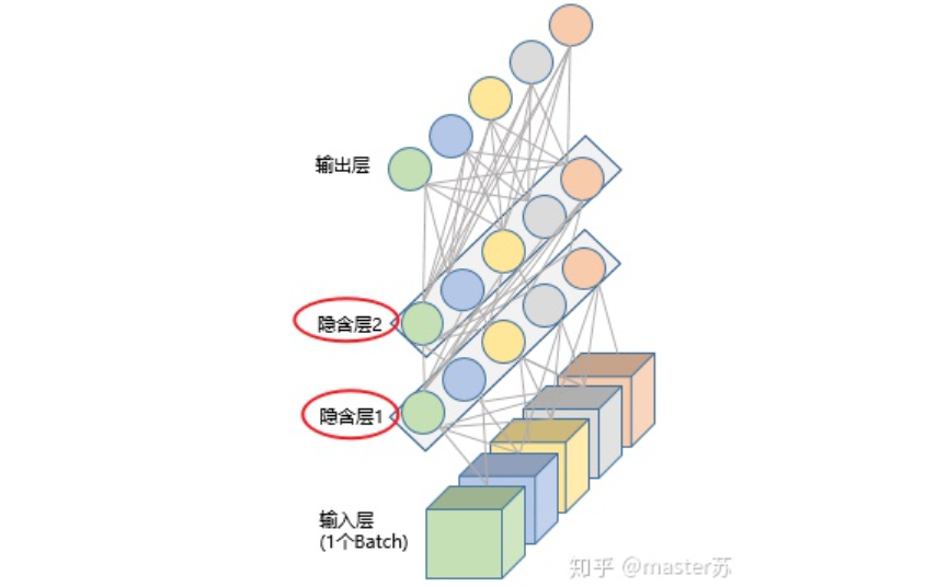
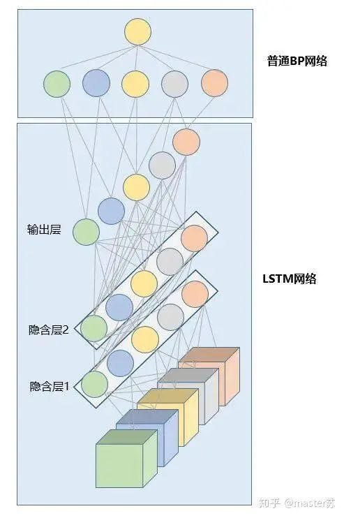
LSTM Network Structure
The above diagram represents an LSTM network with two hidden layers. When viewed at time T=1, it is an ordinary BP network, and at T=2, it is also an ordinary BP network. However, when expanded along the time axis, the hidden layer information H and C trained at T=1 will be passed to the next moment T=2, as shown in the diagram below. The five arrows pointing to the right in the diagram also indicate the transmission of hidden layer states along the time axis.
Note that in the diagram, H represents the hidden layer state, and C is the forget gate, which will be explained later regarding their dimensions.
Input Structure of LSTM
To better understand the structure of LSTM, it is also necessary to understand the input data situation of LSTM. Mimicking the appearance of a 3-channel image, the data cube of multi-sample, multi-feature data at different times with the addition of the time axis is shown in the diagram below:
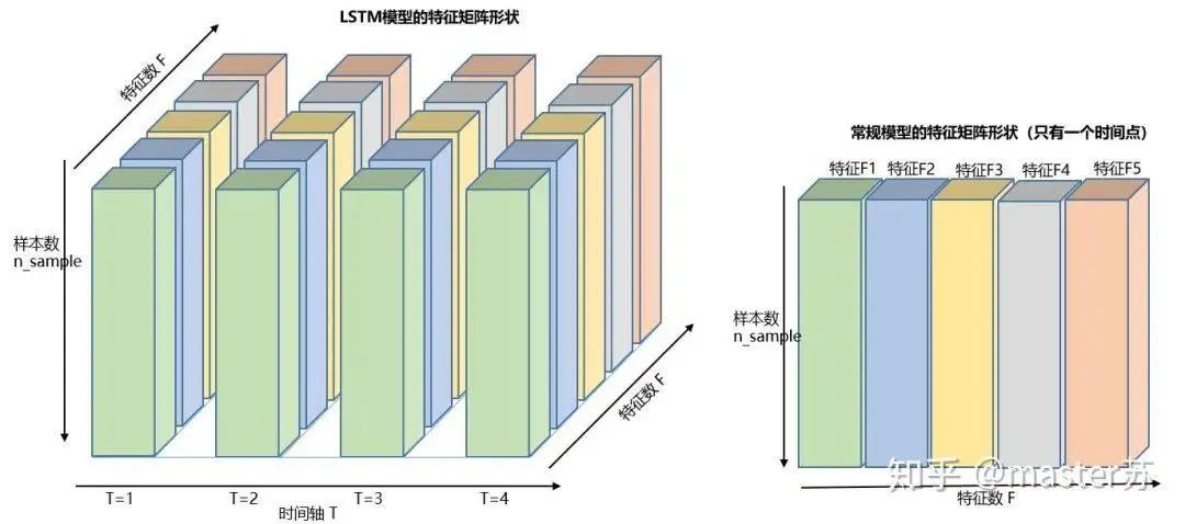
Three-dimensional Data Cube
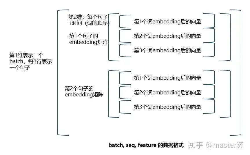
The right diagram shows the input format we commonly use in models such as XGBOOST, lightGBM, decision trees, etc., where the input data format is a matrix of this form (N*F). The left side, however, shows the data cube with the time axis added, which is slices along the time axis. Its dimensions are (N*T*F), where the first dimension is the number of samples, the second dimension is time, and the third dimension is the number of features, as shown in the diagram below:
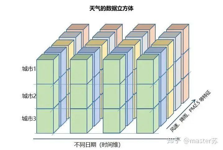
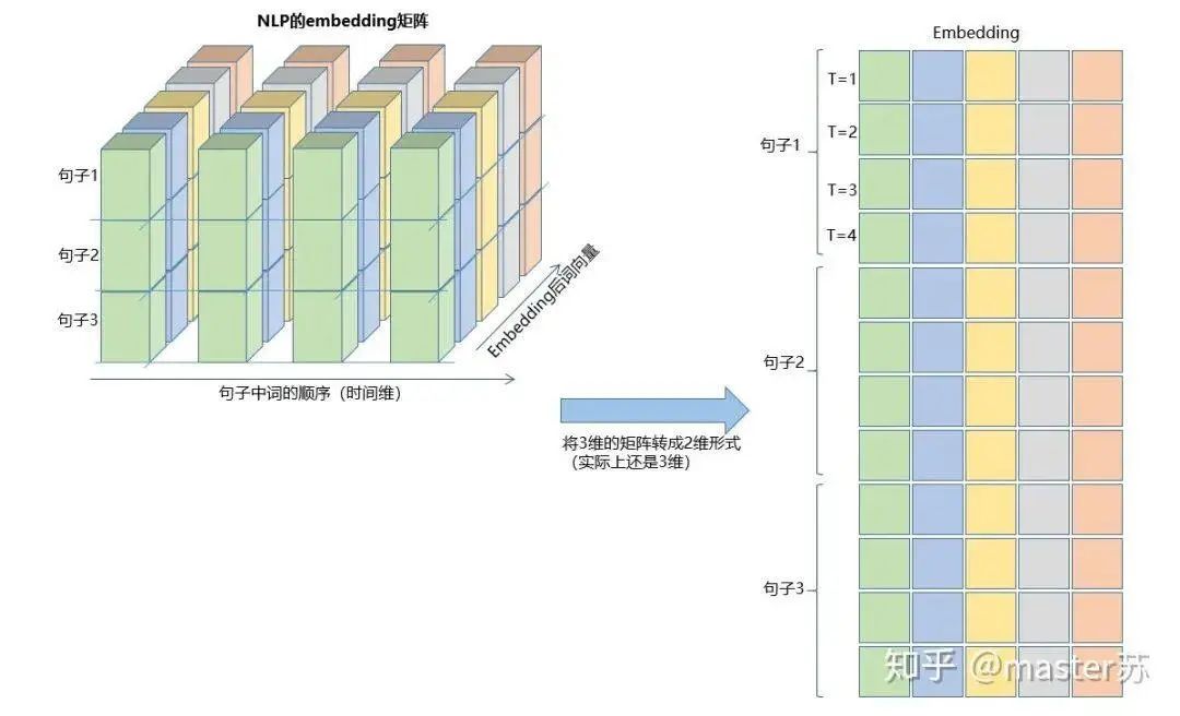
This type of data cube is common in many scenarios, such as weather forecast data, where samples can be understood as cities, the time axis as dates, and features as weather-related factors like rainfall, wind speed, PM2.5, etc. This data cube becomes easy to understand. In NLP, a sentence can be embedded into a matrix, where the order of words represents the time axis T, and the embedding of multiple sentences forms a three-dimensional matrix as shown in the diagram below:

<span>class torch.nn.LSTM(*args, **kwargs)</span><span>Parameters include:</span><span>input_size: Dimension of features in x</span><span>hidden_size: Dimension of the hidden layer's features</span><span>num_layers: Number of LSTM hidden layers, default is 1</span><span>bias: If False, then bihbih=0 and bhhbhh=0. Default is True</span><span>batch_first: If True, then the input/output data format is (batch, seq, feature)</span><span>dropout: Dropout is applied to each layer's output except the last layer, default is 0</span><span>bidirectional: If True, then it is a bidirectional LSTM, default is False</span>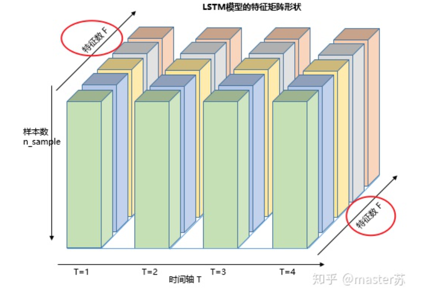
<span>input(seq_len, batch, input_size)</span><span>Parameters include:</span><span>seq_len: Sequence length; in NLP, it is the sentence length, typically padded with pad_sequence to ensure uniform length</span><span>batch: The number of data instances fed to the network at once; in NLP, it is how many sentences are fed to the network at one time</span><span>input_size: Feature dimension, consistent with the input_size defined in the network structure.</span><span>input(batch, seq_len, input_size)</span>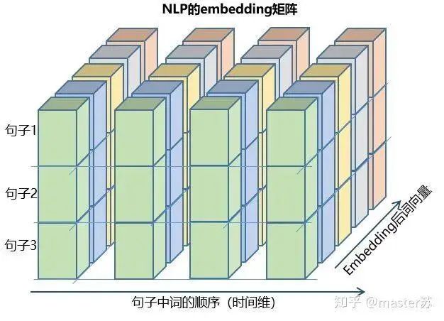
<span>h0(num_layers * num_directions, batch, hidden_size)</span><span>c0(num_layers * num_directions, batch, hidden_size)</span><span>Parameters:</span><span>num_layers: Number of hidden layers</span><span>num_directions: For a unidirectional recurrent network, num_directions=1; for bidirectional, num_directions=2</span><span>batch: Batch of input data</span><span>hidden_size: Number of hidden layer neurons</span><span>input(batch, seq_len, input_size)</span><span>h0(batch, num_layers * num_directions, h, hidden_size)</span><span>c0(batch, num_layers * num_directions, h, hidden_size)</span><span>output,(ht, ct) = net(input)</span><span>output: The output of the hidden layer neurons at the last state</span><span>ht: The state value of the hidden layer at the last state</span><span>ct: The value of the forget gate at the last state of the hidden layer</span><span>output(seq_len, batch, hidden_size * num_directions)</span><span>ht(num_layers * num_directions, batch, hidden_size)</span><span>ct(num_layers * num_directions, batch, hidden_size)</span><span>input(batch, seq_len, input_size)</span><span>ht(batch, num_layers * num_directions, h, hidden_size)</span><span>ct(batch, num_layers * num_directions, h, hidden_size)</span>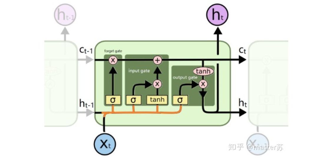
Implementing the above structure in PyTorch:
<span>import torch</span><span>from torch import nn</span><span><span><span>class</span> <span>RegLSTM</span>(<span>nn</span>.<span>Module</span>): </span></span><span><span><span>def</span> <span>__init__</span><span>(<span>self</span>)</span></span>:</span><span> <span>super</span>(RegLSTM, <span>self</span>).__init_<span>_</span>()</span><span> <span># Define LSTM</span></span><span> <span>self</span>.rnn = nn.LSTM(input_size, hidden_size, hidden_num_layers)</span><span> <span># Define regression layer network, input feature dimension equals LSTM's output, output dimension is 1</span></span><span> <span>self</span>.reg = nn.Sequential(</span><span> nn.Linear(hidden_size, <span>1</span>)</span><span> )</span><span> <span><span>def</span> <span>forward</span><span>(<span>self</span>, x)</span></span>:</span><span> x, (ht,ct) = <span>self</span>.rnn(x)</span><span> seq_len, batch_size, hidden_size= x.shape</span><span> x = y.view(-<span>1</span>, hidden_size)</span><span> x = <span>self</span>.reg(x)</span><span> x = x.view(seq_len, batch_size, -<span>1</span>)</span><span> <span>return</span> x</span>Reference links:
https://zhuanlan.zhihu.com/p/94757947
https://zhuanlan.zhihu.com/p/59862381
https://zhuanlan.zhihu.com/p/36455374
https://www.zhihu.com/question/41949741/answer/318771336
https://blog.csdn.net/android_ruben/article/details/80206792
Editor: Wang Jing
Proofreader: Lin Yilin
Reference links can be found at the bottom left corner of the article. For academic sharing only; if there is any infringement, please delete immediately.
Editor /Garvey
Review / Fan Ruiqiang
Verification / Garvey
Click below
Follow us