
Source: Big Data Mining DT Data Analysis
This article is 1500 words, suggested reading time 5 minutes.
This article introduces the principles of LSTM networks and their application in the pop music trend prediction competition.
Reply with the keyword“music” to download the complete code and dataset
1. Principles of LSTM Networks
1.1 Key Points
-
LSTM networks are used to process data with the “sequence” property. For example, time series data, such as daily stock price trends, mechanical vibration signals in the time domain, and natural language data composed of ordered words.
-
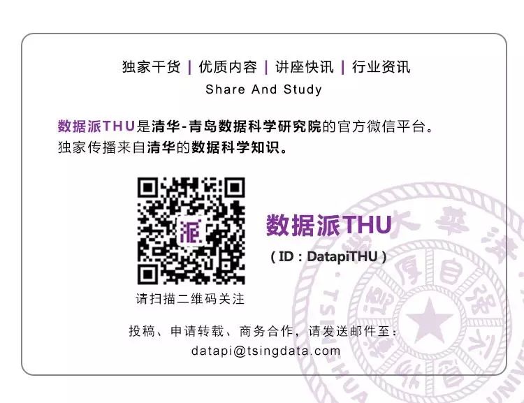
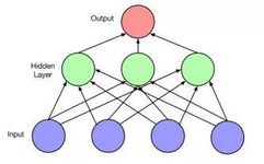
LSTM is not an independent network structure; it is just a part of the entire neural network, where the LSTM structure replaces the hidden layer units in the original network.
-
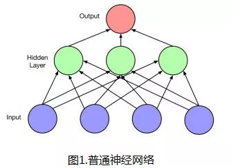
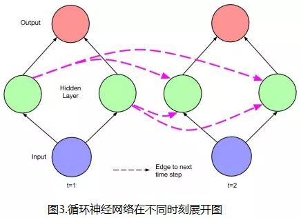
LSTM networks have “memory”. This is because there are connections between the networks at different “time points”, rather than only feedforward or feedback at a single time point. As shown in the LSTM unit (hidden layer unit) in Figure 2. Figure 3 shows the network expansion diagram at different moments. The dashed lines represent time, while the connections of the “network itself” are represented by solid lines.
1.2 Structure Diagram of LSTM Units
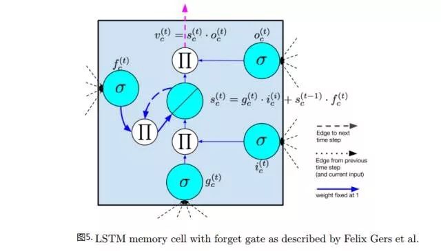
Figures 4 and 5 show the commonly used structure diagrams of LSTM units:
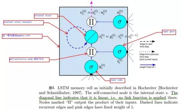
The main structural components include:
-
Input Node input node: accepts the output of the previous hidden layer unit and the current sample input;
-
Input Gate input gate: the input gate multiplies with the input node’s value to form part of the internal state unit value in LSTM. When the gate’s output is 1, the activation value of the input node flows entirely to the internal state. When the gate’s output is 0, the input node’s value has no effect on the internal state.
-
Internal State internal state.
-
Forget Gate forget gate: used to refresh the state of the internal state, controlling the effect of the previous state of the internal state on the current state.
The relationship between each node and gate with the hidden unit output is shown in Figures 4 and 5.
2. Code Example
Reply with the keyword “music” to download the complete code and dataset
Running environment: Windows with Spyder, language: Python 2.7, and Keras deep learning library.
Since I had no Python basics before looking at this competition, I learned Python while thinking about the ideas. I didn’t have much understanding of data structures in Python, so the code is a bit messy. However, the entire code runs correctly. This is also the final version of the code used in the preliminary round.
2.1 Example Introduction
Mainly based on the “2016 Alibaba Pop Music Trend Prediction” competition I participated in this year.
Time flies; today is the last day of the second season. I started engaging with the competition from May 18 until the first season deadline on June 14 at 10 AM. During this period, since it is an offline competition, various models can be used, and I chose to use the LSTM-based recurrent neural network model as I am doing research in deep learning. Fortunately, I made it to the second season. I have been learning deep learning for over half a year now, and it feels rewarding to apply what I learned to a real-life application. I suddenly realized that after so many years of study, my future direction and motivation should be to “learn and apply what I have learned.”
Here is a brief introduction to the competition:
The official provided “input” consists of two tables:
-
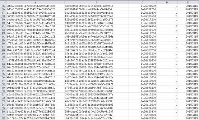
One is the User Behavior Table (time span 20150301-20150830) mars_tianchi_user_actions, mainly describing user behaviors such as collecting, downloading, and playing songs;
-
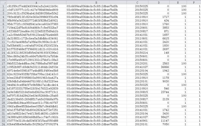
The other is the Song Information Table mars_tianchi_songs, mainly used to describe the artist of the song and related information such as release time, initial popularity, language, etc.
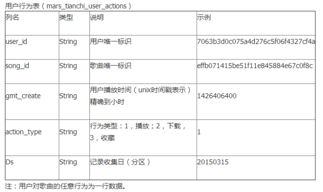
Example:
 Example:
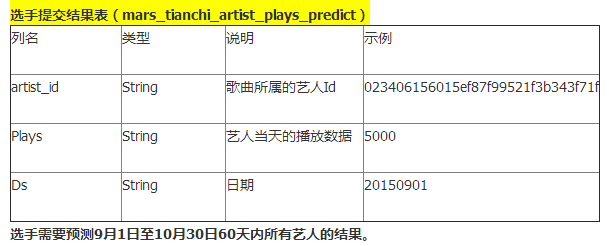
The official requirement for the “output”: predict the daily play volume of each artist for the subsequent two months (20150901-20151030). Output format:
 2.2 Model Approach Used in the Preliminary Round
Since the task is to predict the play volume of artists, I directly related the “play volume” of each artist and observed the trend of play volume changes over the 8 months from 20150301 to 20151030. Using daily play volume, the average play volume over three days, and the variance of play volume over three days as a sample for a time point, I constructed the training set for the neural network. The network structure is as follows:
-
Input Layer: 3 neurons, representing play volume, average play volume, and variance of play volume;
-
First Hidden Layer: LSTM structure unit with 35 LSTM units;
-
Second Hidden Layer: LSTM structure unit with 10 LSTM units;
-
Output Layer: 3 neurons, representing the same meanings as the input layer.
Objective function: reconstruction error.
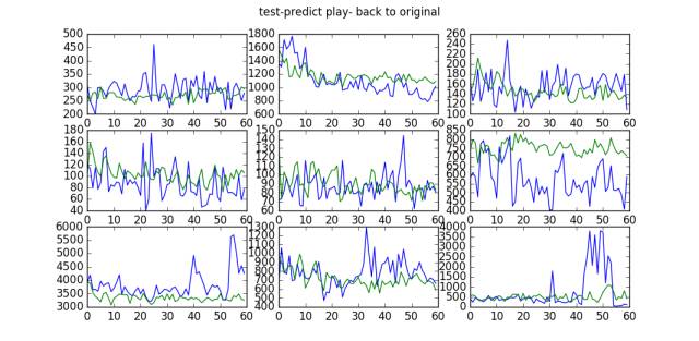
Below is the play statistics curve for certain artists:
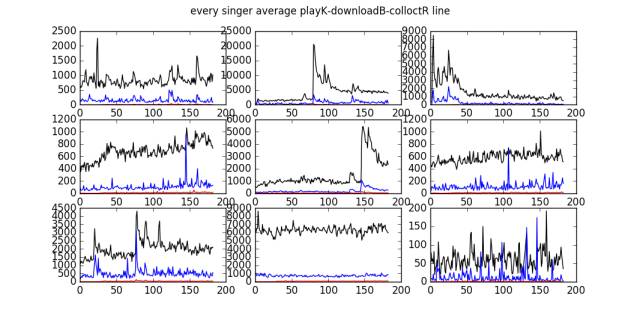
2.2 Prediction Results
The blue line represents the actual play curve of the artist, while the green line represents the predicted curve:
References
-
Good introductory article on LSTM: A Critical Review of RNN for Sequence Learning
-
LSTM learning ideas, see a detailed introduction on Zhihu: https://www.zhihu.com/question /29411132
-
Python introductory video tutorial—see Nanjing University Professor Zhang Li’s public course on Coursera “Using Python to Play with Data”, which includes practical examples: https://www.coursera.org/learn/hipython/home/welcome
-
Keras introduction—see the official documentation
http://keras.io/
Original article link:
http://blog.csdn.net/u012609509/article/details/51910405
Editor: Huang Jiyan