First, I recommend a Jupyter environment, which is provided by Google called colab (https://colab.research.google.com/), where you can use free GPUs.
The first time you use it, you need to download the relevant Python libraries in the experimental environment.
!pip install torch!pip install torchtext!python -m spacy download enOur preliminary idea is to first input a sentence into the LSTM. The number of outputs corresponds to the number of words in the sentence. Then, all outputs are passed through a Linear Layer, where the out_size is 1, serving the purpose of Binary Classification.
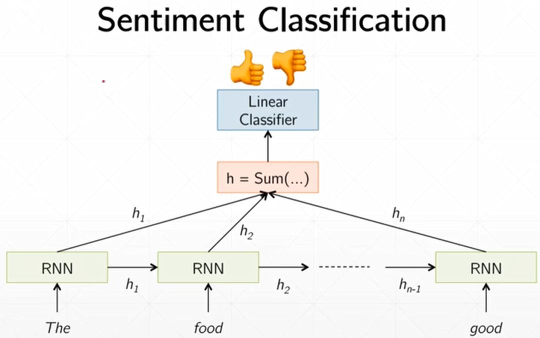
For each input, we need to perform Embedding first, converting each word into a fixed-length vector before sending it into the LSTM. Assuming we represent each word with a vector of length 100, and each sentence has seq words (dynamic, the seq length of each sentence may not be the same), the input shape will be [seq, b, 100]. The final output shape through the Linear Layer will be [b].
The dataset we are using is the IMDB dataset from the torchtext library.
import torch
from torch import nn, optim
from torchtext import data, datasets
print("GPU:", torch.cuda.is_available())
torch.manual_seed(123)
TEXT = data.Field(tokenize='spacy')
LABEL = data.LabelField(dtype=torch.float)
train_data, test_data = datasets.IMDB.splits(TEXT, LABEL)
print('len of train data:', len(train_data))
print('len of test data:', len(test_data))
print(train_data.examples[15].text)
print(train_data.examples[15].label)
# word2vec, glove
TEXT.build_vocab(train_data, max_size=10000, vectors='glove.6B.100d')
LABEL.build_vocab(train_data)
batch_size = 30
device = torch.device('cuda')
train_iterator, test_iterator = data.BucketIterator.splits(
    (train_data, test_data),
    batch_size=batch_size,
    device=device)
Some parameters in the above code may be confusing, but that’s okay since they are just for loading the dataset and are not very important. If you want to learn more about torchtext, you can check this article (https://blog.csdn.net/u012436149/article/details/79310176).
Next, we need to define the network structure, which is quite important.
class RNN(nn.Module):
    def __init__(self, vocab_size, embedding_dim, hidden_dim):
        super(RNN, self).__init__()
        # [0-10001] => [100]
        self.embedding = nn.Embedding(vocab_size, embedding_dim)
        # [100] => [200]
        self.rnn = nn.LSTM(embedding_dim, hidden_dim, num_layers=2,
                           bidirectional=True, dropout=0.5)
        # [256*2] => [1]
        self.fc = nn.Linear(hidden_dim*2, 1)
        self.dropout = nn.Dropout(0.5)

    def forward(self, x):
        # [seq, b, 1] => [seq, b, 100]
        embedding = self.dropout(self.embedding(x))
        # output: [seq, b, hid_dim*2]
        # hidden/h: [num_layers*2, b, hid_dim]
        # cell/c: [num_layers*2, b, hid_dim]
        output, (hidden, cell) = self.rnn(embedding)
        # [num_layers*2, b, hid_dim] => 2 of [b, hid_dim] => [b, hid_dim*2]
        hidden = torch.cat([hidden[-2], hidden[-1]], dim=1)
        # [b, hid_dim*2] => [b, 1]
        hidden = self.dropout(hidden)
        out = self.fc(hidden)
        return out
nn.embedding(m, n) where m represents the total number of words and n represents the dimension of the word embedding (each word is encoded as a vector of length n).
Next is the LSTM itself; I won’t elaborate too much here. You can check my article for parameter introductions (https://wmathor.com/index.php/archives/1400/). One point not mentioned in previous articles is the bidirectional parameter, which, when set to True, indicates that this LSTM is bidirectional. This is easy to understand; the RNNs learned before are unidirectional, which are quite limited. For example, in the sentence below:
-
I am not feeling well today, I plan to ___ for a day
If it is a unidirectional RNN, this blank will definitely be filled with “hospital” or “sleeping”. However, if it is bidirectional, it can know that the next word is “day”, making the probabilities of choosing “take leave” or “rest” much higher.
The final Fully Connected Layer can be understood as integrating all output information into a one-dimensional tensor.
rnn = RNN(len(TEXT.vocab), 100, 256)
pretrained_embedding = TEXT.vocab.vectors
print('pretrained_embedding:', pretrained_embedding.shape)
rnn.embedding.weight.data.copy_(pretrained_embedding)
print('embedding layer initialized.')
If the Embedding layer is not initialized, the generated weights will be random. Therefore, it must be initialized. The weights are obtained by downloading the Glove encoding method, and the downloaded result is actually just a weight, which directly replaces the weights in the embedding using rnn.embedding.weight.data.copy_(pretrained_embedding).
Now let’s see how to train this network.
import numpy as np

def binary_acc(preds, y):
    """  get accuracy  """
    preds = torch.round(torch.sigmoid(preds))
    correct = torch.eq(preds, y).float()
    acc = correct.sum() / len(correct)
    return acc

def train(rnn, iterator, optimizer, criterion):
    avg_acc = []
    rnn.train()
    for i, batch in enumerate(iterator):
        # [seq, b] => [b, 1] => [b]
        pred = rnn(batch.text).squeeze()
        loss = criterion(pred, batch.label)
        acc = binary_acc(pred, batch.label).item()
        avg_acc.append(acc)
        optimizer.zero_grad()
        loss.backward()
        optimizer.step()
        if i % 10 == 0:
            print(i, acc)
    avg_acc = np.array(avg_acc).mean()
    print('avg acc:', avg_acc)
Training is quite simple; you just feed the text in, and it returns an output with a shape of [b, 1]. Using the squeeze() function, the dimension of 1 is removed, and the shape becomes [b], making it convenient for comparison with the label.
Similarly, testing is also very simple.
def eval(rnn, iterator, criterion):
    avg_acc = []
    rnn.eval()
    with torch.no_grad():
        for batch in iterator:
            # [b, 1] => [b]
            pred = rnn(batch.text).squeeze()
            loss = criterion(pred, batch.label)
            acc = binary_acc(pred, batch.label).item()
            avg_acc.append(acc)
    avg_acc = np.array(avg_acc).mean()
    print(">>test:", avg_acc)
Finally, let’s define the loss and optimizer.
optimizer = optim.Adam(rnn.parameters(), lr=1e-3)
criterion = nn.BCEWithLogitsLoss().to(device)
rnn.to(device)
Here, BCEWithLogitsLoss() is mainly used for binary classification problems. nn.BCELoss() is for binary cross-entropy. Both are used for binary classification, but what is the difference? The difference is that BCEWithLogitsLoss combines the Sigmoid layer and BCELoss into one. If you still don’t understand, you can check this blog (https://blog.csdn.net/qq_22210253/article/details/85222093).
ipynb version code (https://github.com/wmathor/file/blob/master/LSTM.ipynb)
py version code (https://github.com/wmathor/file/blob/master/LSTM.py)
For more articles, click on the