Written by丨Zhang Tianrong
He is not the first person to endow neural networks with “memory,” but the long short-term memory network (LSTM) he invented has provided neural networks with longer and practically useful memory. LSTM has long been used by Google, Apple, Amazon, Facebook, etc., to implement functions such as speech recognition and translation. Today, LSTM has become one of the most commercialized achievements in AI…
The Father of “Long Short-Term Memory” – LSTM
Jürgen Schmidhuber (January 17, 1963 – ) is a German computer scientist who completed his undergraduate studies at the Technical University of Munich, Germany. From 2004 to 2009, he served as a professor of artificial intelligence at the University of Lugano in the Italian-speaking part of Switzerland. On October 1, 2021, Schmidhuber officially joined King Abdullah University of Science and Technology as the director of the Artificial Intelligence Institute.
Starting in 1991, Schmidhuber supervised the doctoral thesis of one of his students, Sepp Hochreiter, researching some issues with traditional memory-based recurrent neural networks (RNN). This research led them to co-author a paper on a new type of recurrent neural network in 1997[1], which they named long short-term memory network (LSTM).
At that time, long short-term memory networks did not receive much attention from the industry, and the first paper on LSTM was rejected by the conference and returned by MIT. However, in the following years, long short-term memory networks were widely adopted because they addressed several shortcomings of RNNs.
The LSTM neural network architecture later became the dominant technology for various natural language processing tasks in research and commercial applications during the 2010s. Although its dominance was later replaced by the more powerful Transformer, it still plays an important role in AI technology. In addition to this major contribution, Schmidhuber also achieved a significant acceleration of convolutional neural networks (CNN) on GPUs, making them 60 times faster than equivalent implementations on CPUs. He has also contributed to meta-learning, generative adversarial networks, and more[2].
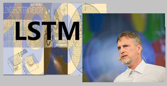 Figure 1:Schmidhuber and LSTM
In 2018, Google Brain researcher David Ha proposed the “World Model” with Schmidhuber, a new method that allows artificial intelligence to predict the future state of the external environment in “dreams,” once again attracting attention.
Although Schmidhuber has made outstanding contributions to AI, compared to the “big three” of deep neural networks in the public’s mind, who are also the three winners of the Turing Award in 2018: Geoffrey Hinton, Yann LeCun, and Yoshua Bengio, his fame is much lower, and he seems to be less appreciated. Some industry insiders believe that Schmidhuber’s own antagonistic personality has led to his significant achievements being underestimated, while Schmidhuber himself has expressed dissatisfaction with many things, believing that his and other researchers’ contributions to deep learning have not been adequately recognized. Schmidhuber has had disagreements with the aforementioned three Turing Award winners and even wrote a “harsh and incisive” article in 2015, stating that the three of them heavily cited each other’s articles and “failed to praise the pioneers in the field,” etc. Later, LeCun denied this accusation, leading to more disputes between the two parties.
However, despite some personality flaws, Schmidhuber is still considered a pioneer in artificial intelligence and is known as the father of LSTM.
Figure 1:Schmidhuber and LSTM
In 2018, Google Brain researcher David Ha proposed the “World Model” with Schmidhuber, a new method that allows artificial intelligence to predict the future state of the external environment in “dreams,” once again attracting attention.
Although Schmidhuber has made outstanding contributions to AI, compared to the “big three” of deep neural networks in the public’s mind, who are also the three winners of the Turing Award in 2018: Geoffrey Hinton, Yann LeCun, and Yoshua Bengio, his fame is much lower, and he seems to be less appreciated. Some industry insiders believe that Schmidhuber’s own antagonistic personality has led to his significant achievements being underestimated, while Schmidhuber himself has expressed dissatisfaction with many things, believing that his and other researchers’ contributions to deep learning have not been adequately recognized. Schmidhuber has had disagreements with the aforementioned three Turing Award winners and even wrote a “harsh and incisive” article in 2015, stating that the three of them heavily cited each other’s articles and “failed to praise the pioneers in the field,” etc. Later, LeCun denied this accusation, leading to more disputes between the two parties.
However, despite some personality flaws, Schmidhuber is still considered a pioneer in artificial intelligence and is known as the father of LSTM.
Traditional RNN Recurrent Neural Networks
Long short-term memory neural networks (LSTM) are an improved class of recurrent neural networks (Recurrent Neural Network or RNN). Therefore, we will first briefly introduce the RNNs before the improvements, or call them “traditional” recurrent neural networks.
Humans have memory, and neural networks certainly need memory too. However, the feedforward neural networks we typically refer to have difficulty simulating memory functions. Feedforward neural networks (Figure 2a) are the most widely used and rapidly developed artificial neural network structure, playing an important role in various application fields during the deep learning era.
In 2001, Bengio et al. introduced probabilistic statistical methods into neural networks, proposing the first language model for neural networks. This model uses a feedforward neural network for language modeling, using a vector of n words as input to predict the probability distribution of the next word through hidden layers. This work laid the foundation for the application of neural networks in natural language processing (NLP).
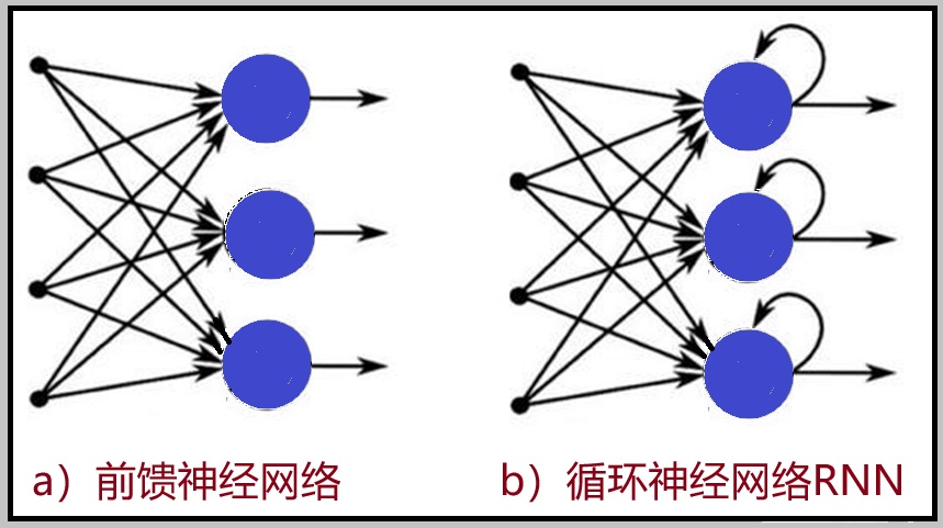 Figure 2:Information flow of feedforward neural networks and recurrent neural networks
Natural language processing (NLP) aims to enable computers to understand and generate human language. Language is a type of time series data, arranged in a sequence over time. When dealing with time series data such as language, a major role of artificial neural networks is to understand the later effects of each input item (vocabulary) and predict what may occur in the future (vocabulary).
Recurrent neural networks (RNN) are the simplest neural networks that simulate human memory capabilities, as shown in Figure 2b.
With the development of deep learning, RNNs began to emerge in the field of NLP. As seen in Figure 2, in the feedforward network, the neurons are arranged in layers, with each neuron only connected to the neurons in the previous layer, receiving the output from the previous layer and outputting to the next layer, with no feedback between layers. In other words, the information in the feedforward network only “moves forward” from input to output. In contrast, RNNs introduce a cyclical structure; they produce output, copy the output, and loop it back into the network. This feedback mechanism allows RNN models to have internal memory, making it easier to handle relationships between items in a data sequence. Figures 2a and 2b illustrate the differences in information flow between feedforward neural networks and RNNs.
In feedforward neural networks, information is never touched by a node more than once, indicating that they have no memory of previously received inputs and thus find it difficult to predict what will happen next. In other words, feedforward networks only consider the current input, so there is no concept of time order, while the state of recurrent neural networks is influenced not only by the input state but also by the previous state. Therefore, recurrent neural networks have a certain memory capability and will remember previous information to apply in the computation of the current output. They are algorithms with internal memory, allowing them to make predictions in continuous data.
The following example can explain the memory concept of RNNs: Suppose you have a feedforward neural network, and you input the sentence “The cake is very sweet” word by word. After processing the first three words, it has already forgotten them, making it difficult to predict the next word “sweet” when processing the word “is.” However, an RNN with memory is very likely to make an accurate prediction.
To better explain how RNNs work, we will illustrate the RNN as shown in Figure 3 (input-output) from bottom to top. We will also unfold the working process of the RNN in chronological order into the sequence shown in Figure 3 (to the right of the equals sign).
In the unfolded RNN sequence, information is gradually passed from one time step to the next. Therefore, RNNs can also be viewed as a network sequence, as shown in the five neural networks after the equals sign in Figure 3, connected in chronological order.
Figure 2:Information flow of feedforward neural networks and recurrent neural networks
Natural language processing (NLP) aims to enable computers to understand and generate human language. Language is a type of time series data, arranged in a sequence over time. When dealing with time series data such as language, a major role of artificial neural networks is to understand the later effects of each input item (vocabulary) and predict what may occur in the future (vocabulary).
Recurrent neural networks (RNN) are the simplest neural networks that simulate human memory capabilities, as shown in Figure 2b.
With the development of deep learning, RNNs began to emerge in the field of NLP. As seen in Figure 2, in the feedforward network, the neurons are arranged in layers, with each neuron only connected to the neurons in the previous layer, receiving the output from the previous layer and outputting to the next layer, with no feedback between layers. In other words, the information in the feedforward network only “moves forward” from input to output. In contrast, RNNs introduce a cyclical structure; they produce output, copy the output, and loop it back into the network. This feedback mechanism allows RNN models to have internal memory, making it easier to handle relationships between items in a data sequence. Figures 2a and 2b illustrate the differences in information flow between feedforward neural networks and RNNs.
In feedforward neural networks, information is never touched by a node more than once, indicating that they have no memory of previously received inputs and thus find it difficult to predict what will happen next. In other words, feedforward networks only consider the current input, so there is no concept of time order, while the state of recurrent neural networks is influenced not only by the input state but also by the previous state. Therefore, recurrent neural networks have a certain memory capability and will remember previous information to apply in the computation of the current output. They are algorithms with internal memory, allowing them to make predictions in continuous data.
The following example can explain the memory concept of RNNs: Suppose you have a feedforward neural network, and you input the sentence “The cake is very sweet” word by word. After processing the first three words, it has already forgotten them, making it difficult to predict the next word “sweet” when processing the word “is.” However, an RNN with memory is very likely to make an accurate prediction.
To better explain how RNNs work, we will illustrate the RNN as shown in Figure 3 (input-output) from bottom to top. We will also unfold the working process of the RNN in chronological order into the sequence shown in Figure 3 (to the right of the equals sign).
In the unfolded RNN sequence, information is gradually passed from one time step to the next. Therefore, RNNs can also be viewed as a network sequence, as shown in the five neural networks after the equals sign in Figure 3, connected in chronological order.
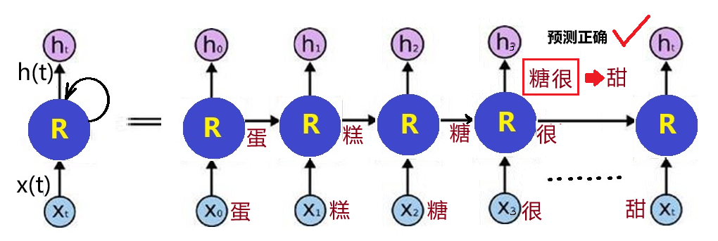 Figure 3:RNN network unfolded into a time series based on its input
As seen in Figure 3, RNNs have two inputs at each time point: the current one and the previous one. Even this “one-time memory” allows RNNs to make predictions that other algorithms cannot make. For example, seeing the words “sugar” and “is,” it is quite possible to predict that the next word is “sweet!”
With the unfolded Figure 3, it is also easy to understand: RNNs can utilize “deep learning” similarly to feedforward networks and adjust weight parameters through gradient descent and backpropagation to train each network layer. However, all concepts here are relative to the “time step.”
Figure 3:RNN network unfolded into a time series based on its input
As seen in Figure 3, RNNs have two inputs at each time point: the current one and the previous one. Even this “one-time memory” allows RNNs to make predictions that other algorithms cannot make. For example, seeing the words “sugar” and “is,” it is quite possible to predict that the next word is “sweet!”
With the unfolded Figure 3, it is also easy to understand: RNNs can utilize “deep learning” similarly to feedforward networks and adjust weight parameters through gradient descent and backpropagation to train each network layer. However, all concepts here are relative to the “time step.”
Weaknesses of RNNs
From the description of traditional RNNs above, it is not difficult to see their weaknesses: the duration of memory is too short! For example, in the above example, it can only remember the previous step. This shortcoming, in AI terminology, is called the “long-term dependency problem.” In other words, traditional recurrent neural networks find it difficult to handle long-distance dependencies because they only possess “short-term memory.”
For instance, if we input a long sentence into the RNN: “Last year I went to Chongqing, learned to cook Sichuan cuisine, particularly loved eating Chongqing’s spicy chicken and boiled beef, in addition, I also learned Chinese, danced Chinese dance, sang Mandarin songs, lived there for half a year, and was extremely happy. Therefore, today in the American restaurant, when I eat this dish, I don’t feel it at all【__].” It is difficult to predict what the word in 【__】 is. We (humans) can easily see that it should be “spicy!” But RNNs struggle to predict it because the relevant information is too far apart.
In other words, RNNs find it difficult to analyze the relationship between input data and information far into the future, and they cannot enhance their predictive capabilities through “learning.” Theoretically, RNNs can learn information from a long time ago by adjusting parameters. However, the conclusion in practice is that RNNs cannot learn information from long ago; the learning process of long-term memory fails for RNNs.
Why can’t they learn? Because when the sequence is too long, recurrent neural networks can encounter “gradient vanishing” or “gradient explosion” issues. Let’s briefly understand this.
Recurrent neural networks use the same method as feedforward networks to “learn” and adjust the network’s weight parameters w. During the machine learning process, backpropagation is used to calculate the gradient of the target function with respect to w.
In simple terms, with each time step the information is passed, the state of the information becomes W times the original. Therefore, after passing n time steps, the information state is W^n times the original. Generally, abs(W)<1, so when n is large, W^n becomes a very small number. This is easy to understand and generally aligns with the facts of the human brain. Because the influence of information on subsequent states is always decreasing, almost forgotten in the end. But unlike the human brain, the repeated stimulation of the same information (learning) can be effective. However, RNN training fails because the very small W^n makes the gradient value too small, and the model stops learning. This is called “gradient vanishing.”
When the algorithm assigns very important values to weights, it can also produce “gradient explosion,” but this situation is rarer. Overall, the gradient vanishing of RNNs is more challenging to solve than gradient explosion.
Long Short-Term Memory (LSTM)
There are many methods to solve the long-term dependency problem, among which the long short-term memory network (LSTM) proposed by Hochreiter and Schmidhuber is a commonly used one.
In fact, the idea of long short-term memory networks is quite simple. It is still analogous to human memory. We often hear that some people have good long-term memory while others have good short-term memory. From a biological perspective, the human brain has two types of memory: long-term and short-term. As mentioned earlier, traditional RNNs already have short-term memory capabilities, so we just need to add a long-term memory function to solve the problem.
Let’s first revisit the short-term memory function of traditional RNNs: we detail the network structure of the unfolded RNN in Figure 3, shown in Figure 4a. The hidden layer of traditional recurrent neural networks has only one state h, which is directly stored at each time step of the network and then input into the next time step, which is the short-term memory.
Now, the idea of LSTM is to add a long-term memory state c, and control c in a certain way to retain memory over a longer period. The newly added state c is called the cell state or memory cell, as shown in Figure 4b.
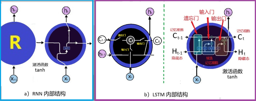 Figure 4:Comparison of the structures of traditional RNNs and LSTM
In the LSTM network, not only is a memory cell c introduced, but also three gate circuits to control it, as shown in Figure 4b. The left side of Figure 4b shows the logical diagram of the relationship between the three gate circuits and the memory cell, while the right side displays a more detailed structure of LSTM.
The first gate of LSTM is called the “forget gate”: besides having long-term memory, the human brain also has the ability to forget. Humans do not need to remember everything they have experienced but only retain important information to reduce the brain’s burden. With memory comes forgetting; forgetting is a special function in memory. The role of the forget gate is to decide what information to discard (forget) from the original memory unit Ct−1 and what information to retain. The forget gate outputs a value between 0 and 1 to the memory cell state Ct−1 through the Sigmoid activation function. 1 means full retention, 0 means complete forgetting, and there are also intermediate values between 0 and 1.
The second is the input gate, which determines whether to send the current instantaneous input information to Ct as long-term memory. Finally, the output gate decides whether to output the information in the current Ct to the next network level.
Thus, from traditional RNNs to LSTM, the cyclical structure remains similar, but the structural elements of the neural network at each “time step” increase from 1 to 4, including one memory cell and three control gates.
LSTM enables RNNs to remember their inputs for long periods, solving the gradient vanishing problem. This is because LSTM incorporates their information into memory (memory cell C), which is very similar to computer memory, as LSTM can read, write, and delete information from memory, and the three control gates can manage these operations. The superiority of AI networks over ordinary computers is that they also possess learning capabilities.
Figure 4:Comparison of the structures of traditional RNNs and LSTM
In the LSTM network, not only is a memory cell c introduced, but also three gate circuits to control it, as shown in Figure 4b. The left side of Figure 4b shows the logical diagram of the relationship between the three gate circuits and the memory cell, while the right side displays a more detailed structure of LSTM.
The first gate of LSTM is called the “forget gate”: besides having long-term memory, the human brain also has the ability to forget. Humans do not need to remember everything they have experienced but only retain important information to reduce the brain’s burden. With memory comes forgetting; forgetting is a special function in memory. The role of the forget gate is to decide what information to discard (forget) from the original memory unit Ct−1 and what information to retain. The forget gate outputs a value between 0 and 1 to the memory cell state Ct−1 through the Sigmoid activation function. 1 means full retention, 0 means complete forgetting, and there are also intermediate values between 0 and 1.
The second is the input gate, which determines whether to send the current instantaneous input information to Ct as long-term memory. Finally, the output gate decides whether to output the information in the current Ct to the next network level.
Thus, from traditional RNNs to LSTM, the cyclical structure remains similar, but the structural elements of the neural network at each “time step” increase from 1 to 4, including one memory cell and three control gates.
LSTM enables RNNs to remember their inputs for long periods, solving the gradient vanishing problem. This is because LSTM incorporates their information into memory (memory cell C), which is very similar to computer memory, as LSTM can read, write, and delete information from memory, and the three control gates can manage these operations. The superiority of AI networks over ordinary computers is that they also possess learning capabilities.
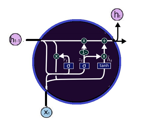 Figure 5:Gated Recurrent Unit (GRU)
The structure shown in Figure 4b is the most typical LSTM structure, and many improvements have been made in practical applications, resulting in various LSTM variants.
For example, the Gated Recurrent Unit (GRU), proposed by Kyunghyun Cho et al. in 2014, is shown in Figure 5. GRU combines the forget gate and the input gate into an “update gate.” It also merges the memory cell state and the hidden state. Studies have found that GRU performs similarly to LSTM in certain tasks such as polyphonic music modeling, speech signal modeling, and natural language processing, but with fewer parameters due to this simplification, making it simpler and more popular than standard LSTM.
Figure 5:Gated Recurrent Unit (GRU)
The structure shown in Figure 4b is the most typical LSTM structure, and many improvements have been made in practical applications, resulting in various LSTM variants.
For example, the Gated Recurrent Unit (GRU), proposed by Kyunghyun Cho et al. in 2014, is shown in Figure 5. GRU combines the forget gate and the input gate into an “update gate.” It also merges the memory cell state and the hidden state. Studies have found that GRU performs similarly to LSTM in certain tasks such as polyphonic music modeling, speech signal modeling, and natural language processing, but with fewer parameters due to this simplification, making it simpler and more popular than standard LSTM.
 References:
[1]Sepp Hochreiter; Jürgen Schmidhuber (1997). “Long short-term memory”. Neural Computation. 9 (8): 1735–1780.
[2]Juergen Schmidhuber’s AI Blog https://people.idsia.ch/~juergen/blog.html
[3]Understanding LSTM Networks: http://colah.github.io/posts/2015-08-Understanding-LSTMs/
[4]Cho, Kyunghyun; van Merrienboer, Bart; Bahdanau, Dzmitry; Bougares, Fethi; Schwenk, Holger; Bengio, Yoshua (2014)