ARIMA/SARIMA vs LSTM: Ensemble Learning for Time Series

Author: Sharmistha Chatterjee

Translator: Chen Zhiyan

Proofreader: Wu Jindi

This article is approximately 5500 words, and it is recommended to read for 10+ minutes.

This article discusses issues related to ensemble learning with simple ARIMA/SARIMA and LSTM time series.

Sharmistha Chatterjee

https://towardsdatascience.com/@sharmi.chatterjee

Motivation

The five most commonly used time series models in traditional time series forecasting are as follows:

Autoregressive (AR) model;
Moving Average (MA) model;
Autoregressive Moving Average (ARMA) model;
Autoregressive Integrated Moving Average (ARIMA);
Seasonal Autoregressive Integrated Moving Average (SARIMA) model.

The Autoregressive AR model linearly represents the current value of the time series using the previous value and the current residual, while the Moving Average MA model linearly represents the current value of the time series using the current value and the previous residual sequence.

The ARMA model is a combination of AR and MA models, where the current value of the time series is linearly represented as its previous values along with the current and previous residual sequences. The time series defined in AR, MA, and ARMA models are all stationary processes, meaning that the mean and covariance between their observations do not change over time.

For non-stationary time series, the series must first be transformed into a stationary stochastic sequence. The ARIMA model is generally suitable for non-stationary time series based on the ARMA model, where the differencing process can effectively convert non-stationary data into stationary data. The SARIMA model, which combines seasonal differencing with the ARIMA model, is used for modeling time series data with periodic characteristics.

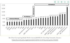
By comparing the performance of these algorithm models in time series, it was found that machine learning methods outperform simple traditional methods, with the overall performance of ETS models and ARIMA models being the best. The following figure compares the models.

However, in addition to traditional time series forecasting, in recent years, recurrent neural networks (RNN) and long short-term memory (LSTM) have been widely applied in various disciplines such as computer vision, natural language processing, and finance in the field of deep learning for time series forecasting. Deep learning methods can identify structures and patterns in data, such as non-linearity and complexity.

Whether the newly developed deep learning-based algorithms for forecasting time series data, such as LSTM, outperform traditional algorithms remains an open question for further research.

The structure of this article is as follows:

Understanding deep learning algorithms RNN, LSTM, and how ensemble learning with LSTM improves performance.
Understanding traditional time series modeling technique ARIMA, and how it improves time series forecasting in ensemble methods when combined with MLP and multiple linear regression.
Understanding the issues and scenarios of using ARIMA with LSTM, comparing their pros and cons. Understanding how to integrate learning with other spatial, decision-based, and event-based models when using SARIMA for time series modeling.

However, this article does not delve deeply into more complex time series issues. For example: complex irregular time structures, missing observations, strong noise, and complex relationships between multiple variables.

LSTM

LSTM is a special type of RNN, composed of a set of cells with features that utilize these features to memorize data sequences, where the cells in the set are used to capture and store the data flow. Additionally, the cells in the set form internal interconnections between the previous module and the current module, thus transmitting information from multiple past time instances to the current module. Each cell uses gates to process, filter, or add data within the cell for the next cell.

The gates in the cells are based on sigmoidal neural network layers, allowing the cells to selectively let data through or discard it; each sigmoid layer outputs a number between 0 and 1, indicating the amount of data that should pass through each cell. More precisely, if this value is 0, it means “do not let any data through,” and if this value is 1, it means “let all data through.” To control the state of each cell, each LSTM involves three types of gates:

Forget Gate outputs a value between 0 and 1, where 1 means “completely retain this value”; and 0 means “completely ignore this value.”
Memory Gate decides which data to pass through the sigmoid layer and the tanh layer to be stored in the data cell. The initial sigmoid layer, known as the “input gate layer,” determines which values need to be modified, and then the tanh layer generates a vector of new candidate values that can be added to the state.
Output Gate decides what content each cell outputs; based on data filtering and the state of the data cell after adding new data, the output gate will output a data value.

In terms of operational principles and implementation mechanisms, the LSTM model provides more fine-tuning options than ARIMA.

Application of LSTM in Time Series Forecasting

Research has found that a single LSTM network trained on a specific dataset is likely to perform poorly on completely different time series; therefore, strict parameter optimization needs to be performed. Due to the success of LSTM in the forecasting domain, researchers have adopted a so-called stacked ensemble method, stacking and combining multiple LSTM networks to provide more accurate predictions, aiming to provide a more universal model for forecasting problems.

By studying four different forecasting problems, it was concluded that the performance of the stacked LSTM network outperforms conventional LSTM networks and ARIMA models based on the RMSE evaluation metric.

By adjusting the parameters of each LSTM, the overall quality of the ensemble method can be improved. The poor performance of a single LSTM network is due to the need to adjust a large number of parameters of the LSTM networks. Therefore, the concept of ensemble LSTM networks has developed, reducing the need for extensive parameter optimization and improving the quality of predictions, thus providing a better choice for forecasting problems.

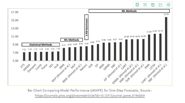
In other ensemble techniques, as shown in the figure above, hybrid ensemble learning with long short-term memory (LSTM) can be used to predict financial time series. The AdaBoost algorithm is used to combine predictions from multiple independent long short-term memory (LSTM) networks.

First, the AdaBoost algorithm is used to train the data, generating replacement samples from the original dataset to obtain training data; then, the LSTM is used to predict each training sample separately; finally, the AdaBoost algorithm is used to integrate the predictions from all LSTM predictors, generating ensemble results. Empirical results on two major daily exchange rate datasets and two stock market index datasets indicate that the AdaBoost-LSTM ensemble learning method outperforms other single prediction models and ensemble learning methods.

The AdaBoost-LSTM ensemble learning method has broad application prospects in predicting financial time series data, and it also shows good application prospects for nonlinear and irregular time series data such as exchange rates and stock indices.

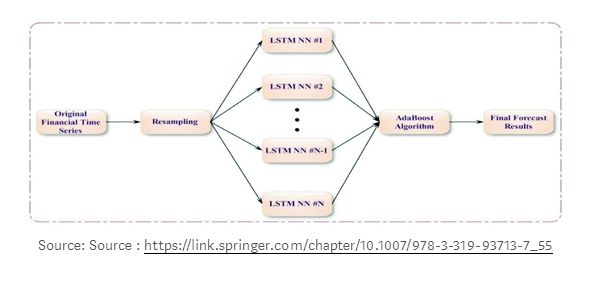
As shown in the figure above, another example of ensemble learning in LSTM is when the input layer contains inputs from time t1 to tn, where each moment’s input is fed into the LSTM layer, and the output of each LSTM layer HK represents partial information at time k, which is input into the output layer, where the output layer aggregates and calculates the mean from all received outputs. Additionally, the mean is input into a logistic regression layer to predict the label of the sample.

ARIMA

The ARIMA algorithm is a class of models for capturing time structures in time series data; however, it is difficult to model nonlinear relationships between variables using the ARIMA model alone.

The Autoregressive Integrated Moving Average (ARIMA) is a generalized Autoregressive Moving Average (ARMA) model that combines the Autoregressive (AR) process and the Moving Average (MA) process, constructing a composite model of the time series.

AR: Autoregressive. A regression model that uses the dependence between one observation and multiple lagged observations.
I: Integrated. Stabilizes the time series by calculating the differences between observations at different times.
MA: Moving Average. A method for calculating the dependency between observations and residual terms when using a moving average model on lagged observations (q). A simple form of the AR model of order p, AR(P), can be expressed as a linear process represented by the following formula:

Here, xt represents the stationary variable, c is a constant, and the terms in ∅t are the autocorrelation coefficients of lag 1, 2, … The residual p and ξt are Gaussian white noise sequences with a mean of zero and a variance of σt².

The general form of the ARIMA model is represented as ARIMA(p, q, d). For seasonal time series data, the short-term non-seasonal part is likely to contribute to the model. The ARIMA model is typically represented as ARIMA(p, q, d), where:

p is the number of lagged observations used when training the model (i.e., the lag order).
d is the number of times differencing is applied (i.e., the order of differencing).
q is the size of the moving average window (i.e., the order of the moving average).

For example, ARIMA(5, 1, 0) indicates that the autoregressive lag values are set to 5, using first-order differencing to stabilize the time series, without considering any moving average window (i.e., the window size is zero). RMSE can be used as an error metric to evaluate the performance of the model and assess the accuracy of predictions.

To this end, we need to utilize the seasonal ARIMA model, which is a composite model that includes both non-seasonal and seasonal factors. The general form of the seasonal ARIMA model can be represented as (p, q, d) X (P, Q, D)S, where p is the non-seasonal AR order, d is the non-seasonal differencing, q is the non-seasonal MA order, P is the seasonal AR order, D is the seasonal differencing, Q is the seasonal MA order, and S is the time span of the repeating seasonal pattern. The most important step in estimating the seasonal ARIMA model is identifying the values of (p, q, d) and (P, Q, D).

According to the time plot of the data, if the variance increases over time, variance-stabilizing transformations and differencing should be applied.

Using the autocorrelation function (ACF) to calculate the linear correlation between observations in the time series separated by p lags, using the partial autocorrelation function (PACF) to determine how many autoregressive terms q are needed, and using the inverse autocorrelation function (IACF) to detect over-differencing, we can obtain the initial values for the autoregressive order p, differencing order d, the moving average order q, and their corresponding seasonal parameters P, D, and Q. The parameter d is the order of frequency change from non-stationary time series to stationary time series.

In the process of applying the univariate method of “Autoregressive Moving Average (ARMA)” to a single time series data, the Autoregressive (AR) model and the Moving Average (MA) model are combined, and the univariate “Differenced Autoregressive Moving Average Model (ARIMA)” is a special ARMA model that considers differencing.

Multivariate ARIMA models and vector autoregressive models (VAR) are two other popular forecasting models that extend the univariate ARIMA model and univariate autoregressive (AR) model by considering multiple evolving variables.

ARIMA is a prediction method based on linear regression, best suited for single-step sample forecasts. Here, the mentioned algorithm is for multi-step sample forecasting and re-estimation, meaning that the model is re-fitted each time to establish the best estimating model. This algorithm builds a forecasting model based on the input “time series” dataset and calculates the mean squared error of the predictions. It stores two data structures to save the accumulated training dataset added at each iteration, namely: the “historical” values and the continuous predictions of the test dataset, the “predicted” values.

Ensemble Learning Based on ARIMA

Training, validating, and testing three forecasting models: ARIMA, multilayer perceptron (MLP), and multiple linear regression (MLR) resulted in predictions of the target pollutant concentration. To train and fit the ARIMA model, the values of p, d, q were estimated using the autocorrelation function (ACF) and the partial autocorrelation function (PACF). The MLP model was established using the following parameters: the solver for weight optimization is lbfgs, as it converges faster and performs better for lower-dimensional data.

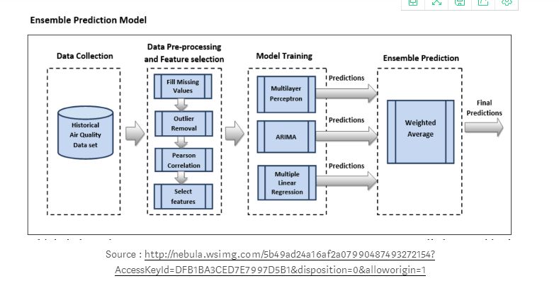
Compared to the stochastic gradient descent optimizer, it achieved better results, utilizing the activation function “relu” to represent the rectified linear unit (RELU) function, thus avoiding the vanishing gradient problem. Then, using a weighted average ensemble technique, the predictions of each model were combined into the final prediction. The weighted average ensemble takes the predictions of each model, multiplies them by their weights, and then calculates the average. The weights of each base model can be adjusted based on the performance of each model.

The predictions of each model are combined using the weighted average technique, where each model is assigned different weights based on its performance, with better-performing models receiving higher weights, and the principle of weight distribution should ensure that the sum of weights equals 1.

SARIMA

ARIMA is one of the most widely used univariate time series forecasting methods, but it does not support time series with seasonal components. To accommodate the seasonal component of the series, the ARIMA model is extended to SARIMA. SARIMA (Seasonal Autoregressive Integrated Moving Average) is applied to univariate data containing trends and seasonality, consisting of sequences made up of trend and seasonal factors.

Some parameters that are the same as the ARIMA model include:

p: the autoregressive order of the trend.
d: the differencing order of the trend.
q: the moving average order of the trend.

Four seasonal factors that are not part of ARIMA include:

P: seasonal autoregressive order.
D: seasonal differencing order.
Q: seasonal moving average order.
m: the number of time steps in a single seasonal cycle.

The SARIMA model can be defined as:

SARIMA (p, d, q) (P,D,Q) m

If m is 12, it specifies a seasonal cycle of monthly data for the year.

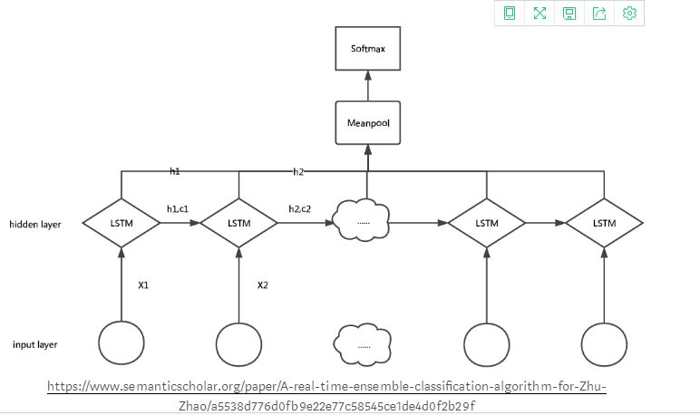
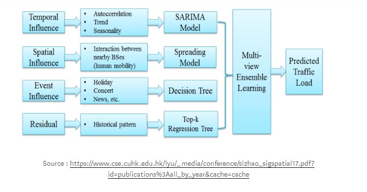
SARIMA time series models can also be combined with spatial and event-based models to generate ensemble models that solve multidimensional ML problems. Such ML models can be used to predict cell loads in cellular networks at different times of the year, as shown in the sample diagram below.

In time series analysis, autocorrelation, trends, and seasonality (weekday, weekend effects) can be used to explain time effects.

The distribution of loads in regions and cells can be used to predict sparse and overloaded units over different time intervals.

Using decision trees to predict events (holidays, special mass gatherings, and other activities).

Dataset, Problem, and Model Selection

When analyzing the problems that classic machine learning and deep learning mechanisms need to solve, the following factors need to be considered before finally selecting the right model.

The different performance metrics of classic time series models (ARIMA/SARIMA) and deep learning models.
The business impact generated by the model selection is long-term or short-term.
The design, implementation, and maintenance costs of more complex models.
The loss of interpretability.

First, the data is highly dynamic, and it is often challenging to sort out the structures embedded within time series data; secondly, time series data can be nonlinear and contain highly complex autocorrelation structures. Data points from different time periods can be interrelated, and linear approximations may not model all structures in the data. Traditional methods, such as autoregressive models, attempt to estimate the parameters of the model, which can be viewed as a smooth approximation of the structure generating the data.

In summary, ARIMA models data with linear relationships better, while RNNs (depending on the activation function) better establish model data with nonlinear relationships. The ARIMA model provides a better choice for data scientists, and later, when the residuals after data are tested by Lee, White, and Granger (LWG) still contain nonlinear relationships, nonlinear models like RNN can further process the dataset.

After applying LSTM and ARIMA to a set of financial data, the results indicate that LSTM outperforms ARIMA, with the average prediction accuracy of the LSTM algorithm improved to 85% compared to ARIMA.

Conclusion

This article concludes with some case studies on why certain machine learning methods perform poorly in practice, yet excel in other areas of artificial intelligence. To this end, this article evaluates the reasons for the poor performance of ARIMA/SARIMA and LSTM models and designs mechanisms to improve model performance and accuracy. The application areas and performance of these models are as follows:

ARIMA has better predictive effects for short-term forecasting, while LSTM has better predictive effects for long-term models.
Traditional time series forecasting methods (ARIMA) focus on univariate data with linear relationships and fixed manual diagnostic time dependencies.
Research on machine learning problems with large datasets found that the average error rate obtained by LSTM ranges from 84-87%, indicating that LSTM outperforms ARIMA.
In deep learning, “epoch” refers to the number of training iterations, which does not affect the performance of the trained prediction model, presenting true randomness.
LSTM seems to be more suitable for fitting or overfitting training datasets rather than predicting datasets compared to simpler NNs like RNN and MLP.
Neural networks with large datasets (LSTMs and other deep learning methods) provide a method to divide them into several smaller batches and train them across multiple stages. The batch size/size of each block is determined by the total number of training data used. The term: iteration refers to the number of batches needed to complete the training of the entire dataset model.
LSTM is undoubtedly more complex and harder to train, and in most cases, its performance does not exceed that of simple ARIMA models.
Traditional methods, such as ETS and ARIMA, are suitable for single-step forecasting of univariate datasets.
Classic methods like Theta and ARIMA excel in multi-step forecasting of univariate datasets.
Classic methods like ARIMA focus on fixed time dependencies: the interrelationships between different time observations, which require analysis and explanation of the number of lagged observations input.
Machine learning and deep learning methods have not yet fulfilled their promise for univariate time series forecasting, and there is still much research to be done in this area.
Neural networks increase the capability to handle noise and nonlinear relationships, and have a fixed number of inputs that can be arbitrarily defined. Furthermore, NNs can output multivariate and multi-step predictions.
Recurrent neural networks (RNNs) increase explicit handling of ordered observations and are capable of learning time dependencies from context. By observing a sequence once over a certain period, RNNs can learn the relevant observations from prior sequences and predict subsequent correlations.
When LSTMs are used to learn correlations in long sequences, they can model complex multivariate sequences without specifying any time window.

References

1. https://journals.plos.org/plosone/article?id=10.1371/journal.pone.0194889

2. https://machinelearningmastery.com/findings-comparing-classical-and-machine-learning-methods-for-time-series-forecasting/

3. https://arxiv.org/pdf/1803.06386.pdf

4. https://pdfs.semanticscholar.org/e58c/7343ea25d05f6d859d66d6bb7fb91ecf9c2f.pdf

5. “Ensemble Recurrent Neural Networks for Robust Time Series Forecasting”, Authors: S.Krstanovic and H.Paulheim, published in “Artificial Intelligence” Issue 34, edited by M.Bramer and M.Petridis, Springer International Publishing, 2017, pp.34-46, ISBN: 978-3-319-71078-5.

6. https://link.springer.com/chapter/10.1007/978-3-319-93713-7_55

7. http://nebula.wsimg.com/5b49ad24a16af2a07990487493272154?AccessKeyId=DFB1BA3CED7E7997D5B1&disposition=0&alloworigin=1

8. https://www.ncbi.nlm.nih.gov/pmc/articles/PMC3641111/

9. Traffic Prediction Based on Energy-Saving Cellular Networks: A Machine Learning Method

https://www.cse.cuhk.edu.hk/lyu/_media/conference/slzhao_sigspatial17.pdf?id=publications%3Aall_by_year&cache=cache

Original Title:

ARIMA/SARIMA vs LSTM with Ensemble Learning Insights for Time Series Data

Original Link:

https://towardsdatascience.com/arima-sarima-vs-lstm-with-ensemble-learning-insights-for-time-series-data-509a5d87f20a

Editor: Wang Jing

Proofreader: Wang Xin

Translator’s Profile

ARIMA/SARIMA vs LSTM: Ensemble Learning for Time Series

Chen Zhiyan, graduated from Beijing Jiaotong University with a master’s degree in Communication and Control Engineering. He has served as an engineer at Great Wall Computer Software and Systems Co., Ltd., and at Datang Microelectronics Technology Co., Ltd. Currently, he is a technical support staff at Beijing Wuyichaoqun Technology Co., Ltd. He is engaged in the operation and maintenance of intelligent translation teaching systems and has accumulated certain experience in artificial intelligence deep learning and natural language processing (NLP). In his spare time, he enjoys translation and creative writing, with translated works including IEC-ISO 7816, Iraq Petroleum Engineering Projects, New Fiscal Taxism Declaration, etc. His Chinese-to-English translation work “New Fiscal Taxism Declaration” was officially published in GLOBAL TIMES. He hopes to join the translation volunteer group of THU Data Party platform in his spare time, to communicate and share with everyone for mutual progress.

Recruitment Information for the Translation Team

Job Content: Requires a meticulous heart to translate selected foreign articles into fluent Chinese. If you are an overseas student in data science/statistics/computer-related fields, or working in related fields abroad, or confident in your foreign language skills, you are welcome to join the translation team.

What You Can Get: Regular translation training to improve volunteers’ translation skills, enhance awareness of cutting-edge data science, and overseas friends can stay in touch with domestic technology application development. The background of THU Data Party’s industry-university-research collaboration brings good development opportunities for volunteers.

Other Benefits: Data scientists from well-known companies, students from Peking University, Tsinghua University, and other prestigious universities, including those abroad, will become your partners in the translation team.

Click on “Read the Original” at the end of the article to join the Data Party team~

Notice for Reprinting

For reprinting, please indicate the author and source prominently at the beginning (Reprinted from: Data Party ID: datapi), and place a prominent QR code for Data Party at the end of the article. For articles with original identification, please send [Article Name – Awaiting Authorized Public Account Name and ID] to the contact email to apply for whitelist authorization and edit as required.

After publication, please provide the link feedback to the contact email (see below). Unauthorized reprints and adaptations will be pursued legally.