
Reference Article: https://www.jianshu.com/p/471d9bfbd72f
Before understanding word2vec, we first need to grasp what One-Hot encoding is, as this simple encoding method is quite useful for handling enumerable features.
Encoding
One-Hot encoding, also known as single valid encoding, uses an N-bit state register to encode N states, where each state has its own independent register bit, and at any time, only one bit is valid. For example, suppose we have four samples (rows), each with three features (columns), as shown in the figure:
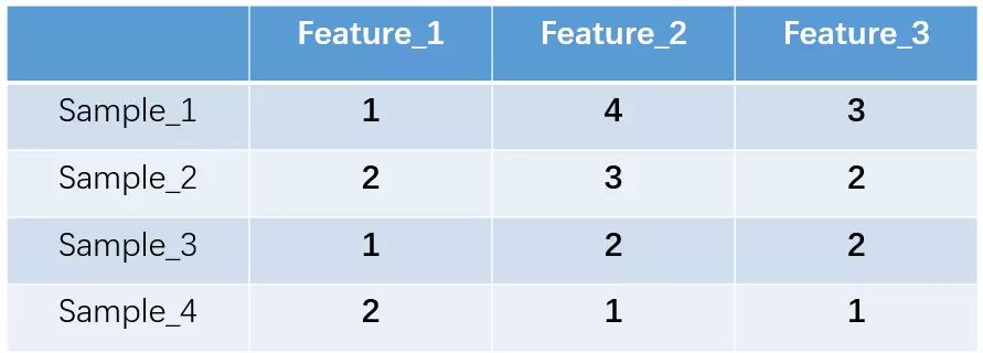
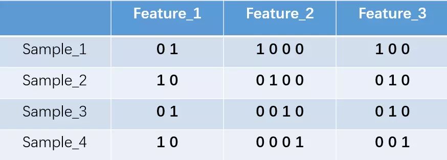
Our feature_1 has two possible values, say male/female, where male is represented by 1 and female by 2. Feature_2 and feature_3 each have four possible values (states). One-hot encoding ensures that in each sample, only one feature is in state 1, while the others are 0. The above states are represented in one-hot encoding as shown below:
In simple terms, the number of possible values for a feature determines the number of binary bits used for representation. Thus, this encoding method is only suitable for enumerable features. For continuous features that cannot be fully enumerated, we need to handle them flexibly, such as treating numbers within a certain range as a single value.
Let’s consider a few examples with three features:
[“male”, “female”]
[“from Europe”, “from US”, “from Asia”]
[“uses Firefox”, “uses Chrome”, “uses Safari”, “uses Internet Explorer”]
After converting to one-hot encoding, it should be:
feature1=[01,10]
feature2=[001,010,100]
feature3=[0001,0010,0100,1000]
Pros and Cons Analysis
• Pros: It addresses the issue where classifiers struggle with discrete data and also helps to some extent in expanding features. • Cons: There are significant shortcomings in text feature representation. Firstly, it is a bag-of-words model that does not consider the order of words (the sequence of words in text is also very important); secondly, it assumes that words are independent of each other (in most cases, words influence each other); finally, the features obtained are discrete and sparse.
Why are the obtained features sparse and discrete?
The examples above are simple, but the reality may differ. For instance, if we consider all city names in the world as the corpus, the resulting vector would be too sparse and would lead to the curse of dimensionality.
Hangzhou [0,0,0,0,0,0,0,1,0,...,0,0,0,0,0,0,0] Shanghai [0,0,0,0,1,0,0,0,0,...,0,0,0,0,0,0,0] Ningbo [0,0,0,1,0,0,0,0,0,...,0,0,0,0,0,0,0] Beijing [0,0,0,0,0,0,0,0,0,...,1,0,0,0,0,0,0]In the corpus, Hangzhou, Shanghai, Ningbo, and Beijing correspond to a vector where only one value is 1, and the rest are 0.
As we can see, when the number of cities is large, the vector representing each city becomes very long, leading to significant wastage since many zeros are almost useless.
A straightforward method to reduce dimensions is to use techniques like PCA, where the features after dimensionality reduction will not be binary but represented as decimal values, allowing for a low dimensionality to cover a large feature space.
Of course, there are many dimensionality reduction methods, and what we are discussing, word2vec, is one of them.
When it comes to word2vec, we first need to understand the neural network-based autoencoder model briefly. An autoencoder is essentially a dimensionality reduction method. The basic structure of an autoencoder network is as follows:
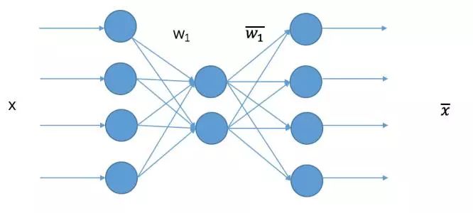
The input to the network is a set of features, which in this case corresponds to a series of 0-1 strings, with the output dimension matching the input dimension. There is a hidden layer mapping in the middle, and our goal is to train the network so that the output X is as close as possible to the input X. Once trained, any input x entering the model can yield the output from the hidden layer, which can be considered the reduced-dimensional representation. As shown in the diagram, this is a network model that reduces from 4 dimensions to 2 dimensions.
Having discussed autoencoders, let’s look at what word2vec is.
Since word2vec is applied in NLP, it encodes words, and a significant feature of NLP is that the representation of a word in a sentence is context-dependent. In other words, this representation is influenced by the temporal order and relative sequence. Thus, word2vec aims to achieve dimensionality reduction while considering the order of words.
How does it solve this? It starts with a basic neural network autoencoder model:
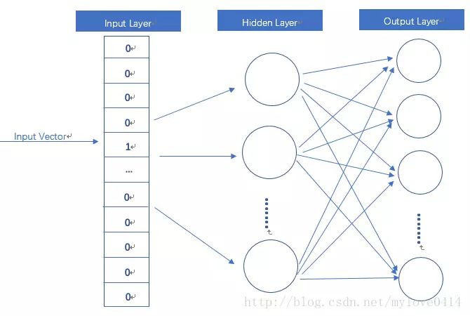
So how do we incorporate contextual information? It’s simple; instead of inputting just one word, we input multiple words from the context:
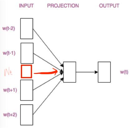
This is a many-to-one model (CBOW), and there is also a one-to-many (Skip-Gram) model. We will first discuss this many-to-one model.
The training model for CBOW is illustrated below:
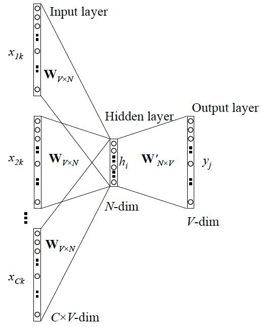
At first glance, it might seem confusing, but it’s essential to understand that this network structure is essentially the original autoencoder network, just that its inputs are not processed all at once but in several batches, and the hidden layer results are the weighted averages of several batches of inputs.
The detailed process is as follows:
1. Input Layer: One-hot of context words.
2. These one-hot vectors are multiplied by shared input weight matrix W.
3. The resulting vectors are summed and averaged to form the hidden layer vector.
4. Multiply by the output weight matrix W {NV}.
5. Obtain the output vector.
6. Compare the output vector with the true one-hot of the word, aiming for minimal error.
This is how the network can be trained. After training, the vector obtained by multiplying each word in the input layer with matrix W is the desired word vector (word embedding). This matrix (the word embeddings for all words) is also referred to as the lookup table (in fact, this lookup table is matrix W itself). This means that any one-hot of a word multiplied by this matrix will yield its word vector. With the lookup table, we can directly look up the word vector without going through the training process.
Compared to the original autoencoder, the most significant difference in word2vec lies in the input, which must consider the sequence of words in the autoencoder. This point is worth understanding well.
This is the many-to-one approach; there is also a one-to-many approach: similarly, the goal is to maintain the order of context while achieving dimensionality reduction.
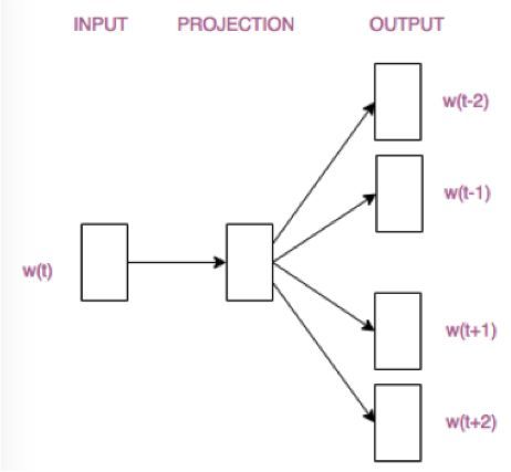
Ultimately, for word2vec training, we need the weight matrix obtained from training. With this weight matrix, we can achieve dimensionality reduction of the input word’s one-hot, while this reduction also incorporates the sequence of context. This is word2vec.
Recommended Reading
Professor Shi Yigong’s Three Female Students: Three Talented Women from One Master, Scientific Achievements Share the Same Sky
Transformer Chatbot Tutorial
Don’t Miss This Wave of Discounts, This Year’s Best!