Summary of Word2Vec in Natural Language Processing

This is a relatively early summary article. Although the content is simple, I personally find it easy to understand. Word2Vec is the cornerstone of natural language processing technology, and a deep understanding of the principles of Word2Vec is crucial for NLP practitioners.

For a long time, I have been unclear about the implementation reasons behind Word2Vec. Therefore, I decided to read two original papers. After finishing, I still felt somewhat confused, so I combined some good explanations found online ( Word2Vec Tutorial – The Skip-Gram Model^[1]), and understood it again with the help of open-source implementation code. Here is a summary.

Below, I will mainly introduce the Word2Vec model.

Word2Vec Workflow

1. It is just a three-layer neural network.
2. Feed a word to the model and use it to predict the surrounding words.
3. Then remove the last layer, keeping the input and output.
4. Select a word from the vocabulary, feed it to the model, and it will provide the output for that word.

import numpy as np
import tensorflow as tf
corpus_raw = 'He is the king . The king is royal . She is the royal  queen '
# convert to lower case
corpus_raw = corpus_raw.lower()

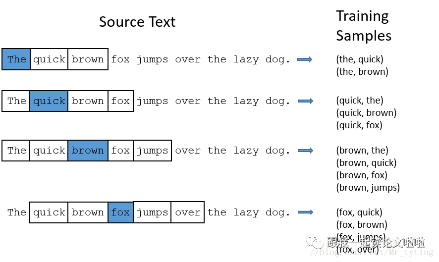
The above code is very simple and easy to understand. Now we need to obtain the surrounding words. Suppose we have a task to feed a word to the model and we need to get its surrounding words. For example, we want to get the words before and after it, as shown in the code:

Note: If the word is at the beginning or end of a sentence, ignore the words outside the window.

We need to perform simple preprocessing on the text data, creating a dictionary of words and their corresponding indices.

words = []
for word in corpus_raw.split():
    if word != '.': # because we don't want to treat . as a word
        words.append(word)
words = set(words) # so that all duplicate words are removed
word2int = {}
int2word = {}
vocab_size = len(words) # gives the total number of unique words
for i,word in enumerate(words):
    word2int[word] = i
    int2word[i] = word

Let’s see what effect this dictionary has:

print(word2int['queen'])
# > 42 (say)
print(int2word[42])
# > 'queen'

Now we can obtain the training data.

data = []
WINDOW_SIZE = 2
for sentence in sentences:
    for word_index, word in enumerate(sentence):
        for nb_word in sentence[max(word_index - WINDOW_SIZE, 0) : min(word_index + WINDOW_SIZE, len(sentence)) + 1] :
            if nb_word != word:
                data.append([word, nb_word])

The above code segments the sentences and words to produce training samples, where the input to the model is a word and the output is a surrounding word.

Shall we print it out and take a look?

print(data)
[['he', 'is'],
 ['he', 'the'],
 ['is', 'he'],
 ['is', 'the'],
 ['is', 'king'],
 ['the', 'he'],
 ['the', 'is'],
 ['the', 'king'],
 .
 .
 .]

Now we have the training data, but we need to convert it into a form that the model can read and understand. This is where the dictionary comes into play.

Let’s further process the data and convert it into vectors:

i.e.,
say we have a vocabulary of 3 words : pen, pineapple, apple
where
word2int['pen'] -> 0 -> [1 0 0]
word2int['pineapple'] -> 1 -> [0 1 0]
word2int['apple'] -> 2 -> [0 0 1]

So why are these called features? I will explain later.

# function to convert numbers to one hot vectors
def to_one_hot(data_point_index, vocab_size):
    temp = np.zeros(vocab_size)
    temp[data_point_index] = 1
    return temp
x_train = [] # input word
y_train = [] # output word
for data_word in data:
    x_train.append(to_one_hot(word2int[ data_word[0] ], vocab_size))
    y_train.append(to_one_hot(word2int[ data_word[1] ], vocab_size))
# convert them to numpy arrays
x_train = np.asarray(x_train)
y_train = np.asarray(y_train)

Building the Model

# making placeholders for x_train and y_train
x = tf.placeholder(tf.float32, shape=(None, vocab_size))
y_label = tf.placeholder(tf.float32, shape=(None, vocab_size))

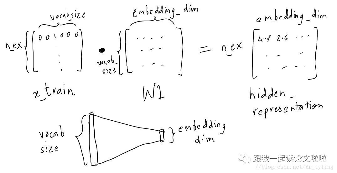
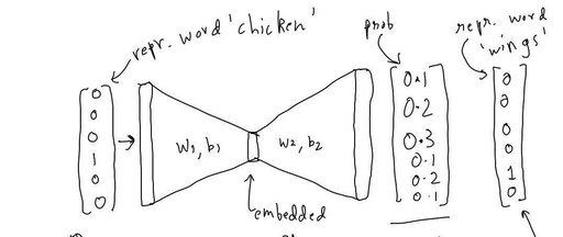
From the above image, we can see that we will convert the input into an embedded representation and reduce the dimensionality to the specified size.

EMBEDDING_DIM = 5 # you can choose your own number
W1 = tf.Variable(tf.random_normal([vocab_size, EMBEDDING_DIM]))
b1 = tf.Variable(tf.random_normal([EMBEDDING_DIM])) #bias
hidden_representation = tf.add(tf.matmul(x,W1), b1)

Next, we need to use this function to predict the surrounding words.

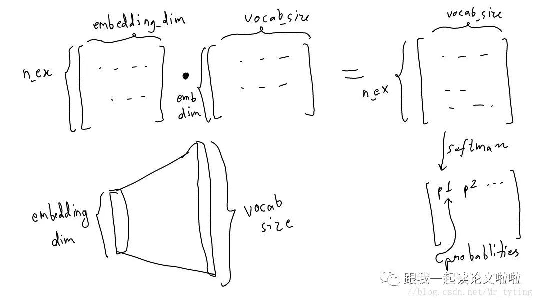
W2 = tf.Variable(tf.random_normal([EMBEDDING_DIM, vocab_size]))
b2 = tf.Variable(tf.random_normal([vocab_size]))
prediction = tf.nn.softmax(tf.add( tf.matmul(hidden_representation, W2), b2))

So the overall process is as follows:

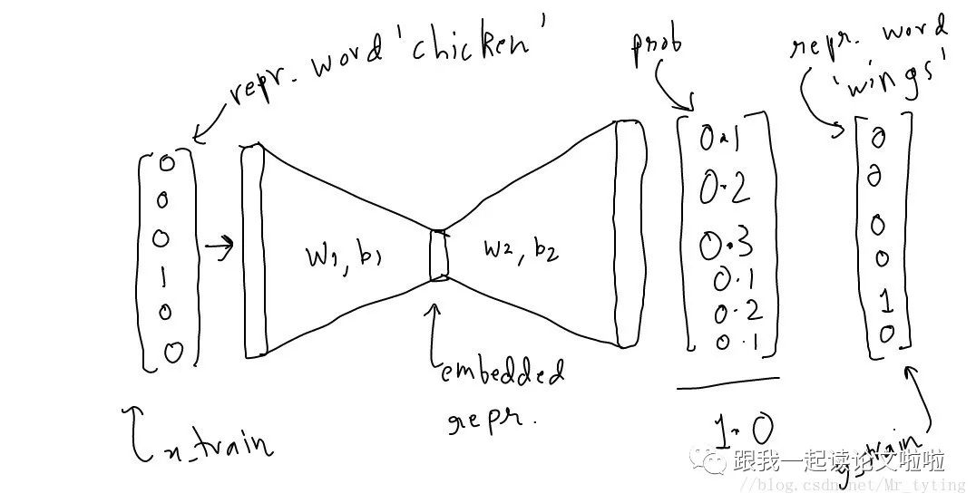
input_one_hot  --->  embedded repr. ---> predicted_neighbour_prob
predicted_prob will be compared against a one hot vector to correct it.

Alright, let’s see how to train this model.

sess = tf.Session()
init = tf.global_variables_initializer()
sess.run(init) #make sure you do this!
# define the loss function:
cross_entropy_loss = tf.reduce_mean(-tf.reduce_sum(y_label * tf.log(prediction), reduction_indices=[1]))
# define the training step:
train_step = tf.train.GradientDescentOptimizer(0.1).minimize(cross_entropy_loss)
n_iters = 10000
# train for n_iter iterations
for _ in range(n_iters):
    sess.run(train_step, feed_dict={x: x_train, y_label: y_train})
    print('loss is : ', sess.run(cross_entropy_loss, feed_dict={x: x_train, y_label: y_train}))

During training, you can see the changes:

loss is :  2.73213
loss is :  2.30519
loss is :  2.11106
loss is :  1.9916
loss is :  1.90923
loss is :  1.84837
loss is :  1.80133
loss is :  1.76381
loss is :  1.73312
loss is :  1.70745
loss is :  1.68556
loss is :  1.66654
loss is :  1.64975
loss is :  1.63472
loss is :  1.62112
loss is :  1.6087
loss is :  1.59725
loss is :  1.58664
loss is :  1.57676
loss is :  1.56751
loss is :  1.55882
loss is :  1.55064
loss is :  1.54291
loss is :  1.53559
loss is :  1.52865
loss is :  1.52206
loss is :  1.51578
loss is :  1.50979
loss is :  1.50408
loss is :  1.49861
.
.
.

Eventually, it will converge. Even if it cannot reach a high level, we do not care about that; our ultimate goal is to obtain good embeddings and representations.

Why Embeddings?

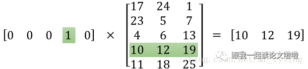
When we multiply the vector by W, we obtain a specific row of the matrix; thus, W acts as a lookup table.

In our code example, we can see the embeddings in the matrix.

print(vectors[ word2int['queen'] ])
# say here word2int['queen'] is 2
# >
[-0.69424796 -1.67628145  3.07313657 -1.14802659 -1.2207377 ]

Given a vector, we can find the closest vector to it.

def euclidean_dist(vec1, vec2):
    return np.sqrt(np.sum((vec1-vec2)**2))

def find_closest(word_index, vectors):
    min_dist = 10000 # to act like positive infinity
    min_index = -1
    query_vector = vectors[word_index]
    for index, vector in enumerate(vectors):
        if euclidean_dist(vector, query_vector) < min_dist and not np.array_equal(vector, query_vector):
            min_dist = euclidean_dist(vector, query_vector)
            min_index = index
    return min_index

Let’s see the closest words:

print(int2word[find_closest(word2int['king'], vectors)])
print(int2word[find_closest(word2int['queen'], vectors)])
print(int2word[find_closest(word2int['royal'], vectors)])
# >
queen
king
he

Advanced Topics

The above summary mainly covers the content of the first paper. Although it is just a three-layer neural network, under massive training data, it requires enormous computational resources to support the entire process. For example, if we set the vocab_size to N, and if N is large, then the matrix dimensions will reach a point where it becomes very slow to optimize the training process. However, sometimes you must use a large amount of data to train the model to avoid overfitting. The paper introduces several solutions.

• Downsampling: Use downsampling to reduce the number of training samples. In the implementation, not all words are used; instead, we first count the frequency of all words and select the top frequent words as the vocabulary. For specific operations, please refer to the code tensorflow/examples/tutorials/word2vec/word2vec_basic.py^[2], and the rest of the words are replaced.

• Negative Sampling: This operation allows a sample to update only a small part of the weight matrix each time, reducing computational pressure during training. For example, if we have a vector, as analyzed above, it is a one-hot vector where only one position is 1 and the rest are 0, and the length of this vector is V. Therefore, each sample can slowly update the weight matrix, while the negative sampling operation randomly selects the remaining parts to make their positions 0, which means we only update the corresponding positions of the weights. For instance, if we choose the number of negative samples to be 5, we select 5 others to make their corresponding positions 0, so we only need to update parameters instead of V parameters.

• Hierarchical Softmax: This is a commonly used method in NLP. For details, please refer to Hierarchical Softmax ^[3]. The main idea is to construct a Huffman tree based on word frequency, where the leaf nodes represent the words in the vocabulary, and higher frequency words are closer to the root node. When calculating the probability of generating a word, we do not need to calculate the probabilities for all words but rather follow the path from the root node to the node where the word is located in the Huffman tree, thus reducing the time complexity from O(N) to O(logN) (where N is the number of nodes, and the depth of the tree is logN).

Personal Summary

• The seq2seq model multiplies at the input and output, and these two embedding matrices may sometimes share parameters and sometimes not. I believe that Word2Vec is actually the prototype of the seq2seq model, just applied to different complex scenarios, adding mechanisms like attention according to the needs of the scene, but the general framework remains.
• Word2Vec is the most fundamental knowledge in the field of natural language processing, and deeply understanding the principles of Word2Vec is crucial.

Complete code:

import tensorflow as tf
import numpy as np

corpus_raw = 'He is the king . The king is royal . She is the royal  queen '

# convert to lower case
corpus_raw = corpus_raw.lower()

words = []
for word in corpus_raw.split():
    if word != '.': # because we don't want to treat . as a word
        words.append(word)

words = set(words) # so that all duplicate words are removed
word2int = {}
int2word = {}
vocab_size = len(words) # gives the total number of unique words

for i,word in enumerate(words):
    word2int[word] = i
    int2word[i] = word

# raw sentences is a list of sentences.
raw_sentences = corpus_raw.split('.');
sentences = []
for sentence in raw_sentences:
    sentences.append(sentence.split())

WINDOW_SIZE = 2

data = []
for sentence in sentences:
    for word_index, word in enumerate(sentence):
        for nb_word in sentence[max(word_index - WINDOW_SIZE, 0) : min(word_index + WINDOW_SIZE, len(sentence)) + 1] :
            if nb_word != word:
                data.append([word, nb_word])

# function to convert numbers to one hot vectors
def to_one_hot(data_point_index, vocab_size):
    temp = np.zeros(vocab_size)
    temp[data_point_index] = 1
    return temp

x_train = [] # input word
y_train = [] # output word

for data_word in data:
    x_train.append(to_one_hot(word2int[ data_word[0] ], vocab_size))
    y_train.append(to_one_hot(word2int[ data_word[1] ], vocab_size))

# convert them to numpy arrays
x_train = np.asarray(x_train)
y_train = np.asarray(y_train)

# making placeholders for x_train and y_train
x = tf.placeholder(tf.float32, shape=(None, vocab_size))
y_label = tf.placeholder(tf.float32, shape=(None, vocab_size))

EMBEDDING_DIM = 5 # you can choose your own number
W1 = tf.Variable(tf.random_normal([vocab_size, EMBEDDING_DIM]))
b1 = tf.Variable(tf.random_normal([EMBEDDING_DIM])) #bias
hidden_representation = tf.add(tf.matmul(x,W1), b1)

W2 = tf.Variable(tf.random_normal([EMBEDDING_DIM, vocab_size]))
b2 = tf.Variable(tf.random_normal([vocab_size]))
prediction = tf.nn.softmax(tf.add( tf.matmul(hidden_representation, W2), b2))

sess = tf.Session()
init = tf.global_variables_initializer()
sess.run(init) #make sure you do this!

# define the loss function:
cross_entropy_loss = tf.reduce_mean(-tf.reduce_sum(y_label * tf.log(prediction), reduction_indices=[1]))

# define the training step:
train_step = tf.train.GradientDescentOptimizer(0.1).minimize(cross_entropy_loss)
n_iters = 10000
# train for n_iter iterations

for _ in range(n_iters):
    sess.run(train_step, feed_dict={x: x_train, y_label: y_train})
    print('loss is : ', sess.run(cross_entropy_loss, feed_dict={x: x_train, y_label: y_train}))

vectors = sess.run(W1 + b1)

def euclidean_dist(vec1, vec2):
    return np.sqrt(np.sum((vec1-vec2)**2))

def find_closest(word_index, vectors):
    min_dist = 10000 # to act like positive infinity
    min_index = -1
    query_vector = vectors[word_index]
    for index, vector in enumerate(vectors):
        if euclidean_dist(vector, query_vector) < min_dist and not np.array_equal(vector, query_vector):
            min_dist = euclidean_dist(vector, query_vector)
            min_index = index
    return min_index

from sklearn.manifold import TSNE

model = TSNE(n_components=2, random_state=0)
np.set_printoptions(suppress=True)
vectors = model.fit_transform(vectors)

from sklearn import preprocessing

normalizer = preprocessing.Normalizer()
vectors =  normalizer.fit_transform(vectors, 'l2')

print(vectors)

import matplotlib.pyplot as plt


fig, ax = plt.subplots()
print(words)
for word in words:
    print(word, vectors[word2int[word]][1])
    ax.annotate(word, (vectors[word2int[word]][0],vectors[word2int[word]][1] ))
plt.show()

References