Hello everyone, I am Xiaohan.
Today, I will share a powerful algorithm model, KNN.
KNN (K-Nearest Neighbors) is an instance-based supervised learning algorithm widely used in classification and regression tasks. Its core idea is: given a sample, calculate its distance to all samples in the training set, find the K nearest samples (the nearest neighbors), and then predict the label of the sample based on the labels of these neighbors.
The Principle of KNN Algorithm
The core idea of KNN is to classify a given sample based on the categories (or values) of the K nearest neighbors in the training set, predicting through voting (for classification) or averaging (for regression). The main steps are as follows:
Calculate Distance
The first step of the KNN algorithm is to calculate the distance between samples. Common distance metrics include:
-
Euclidean Distance
Given two samples and , the Euclidean distance is defined as:
-
Manhattan Distance
The Manhattan distance calculates the sum of the absolute differences between dimensions.
-
Cosine Similarity
Measures the directional similarity between two vectors.
Where the dot product of the vectors is:
Select the K Nearest Neighbors
Select the K data points that are closest.
Voting or Averaging
-
Classification Task
In the KNN classification task, given a sample x to be classified, first calculate its distance to all training samples, then select the K nearest samples and use the majority voting principle to determine the category.
Where:
-
denotes the K nearest neighbors of x -
is an indicator function; if the sample belongs to category , it takes the value 1, otherwise it takes 0 -
Regression Task
In the KNN regression task, the predicted value is usually the average or weighted average of the K neighbors.
Alternatively, a weighting method can be used (such as inverse distance weighting).
Advantages and Disadvantages of KNN
Advantages
-
Simple to implement, easy to understand and execute. -
No special assumptions about data distribution, it is a non-parametric algorithm. -
Applicable to multi-class and regression problems.
Disadvantages
-
High computational complexity; when querying new samples, a large number of distances need to be calculated, with a time complexity of (n is the number of samples, d is the feature dimension). -
Sensitive to noisy data; the choice of K can affect the results. -
In high-dimensional data, the effectiveness of distance calculations may be affected by the “curse of dimensionality”.
Case Study
Below is an example code for classification using the KNN algorithm.
import numpy as np
import matplotlib.pyplot as plt
from sklearn import datasets
from sklearn.model_selection import train_test_split
from sklearn.preprocessing import StandardScaler
from sklearn.neighbors import KNeighborsClassifier
from sklearn.metrics import accuracy_score, classification_report, confusion_matrix
from matplotlib.colors import ListedColormap

# 1. Load the Iris dataset
iris = datasets.load_iris()
X = iris.data[:, :2]  # Select the first two features for visualization
y = iris.target

# 2. Split into training and testing sets
X_train, X_test, y_train, y_test = train_test_split(X, y, test_size=0.2, random_state=42, stratify=y)

# 3. Standardize the data
scaler = StandardScaler()
X_train = scaler.fit_transform(X_train)
X_test = scaler.transform(X_test)

# 4. Train the KNN classifier
k = 5
knn = KNeighborsClassifier(n_neighbors=k, metric='euclidean')
knn.fit(X_train, y_train)

# 5. Predict the test set
y_pred = knn.predict(X_test)

# 6. Evaluate the model
accuracy = accuracy_score(y_test, y_pred)
print(f"KNN classification accuracy: {accuracy:.2f}")
conf_matrix = confusion_matrix(y_test, y_pred)

# 7. Visualize the confusion matrix
plt.figure(figsize=(6, 6))
plt.imshow(conf_matrix, cmap='Blues', interpolation='nearest')
plt.title("Confusion Matrix")
plt.colorbar()
plt.xticks(ticks=[0,1,2], labels=iris.target_names)
plt.yticks(ticks=[0,1,2], labels=iris.target_names)
plt.xlabel("Predicted Label")
plt.ylabel("True Label")
plt.show()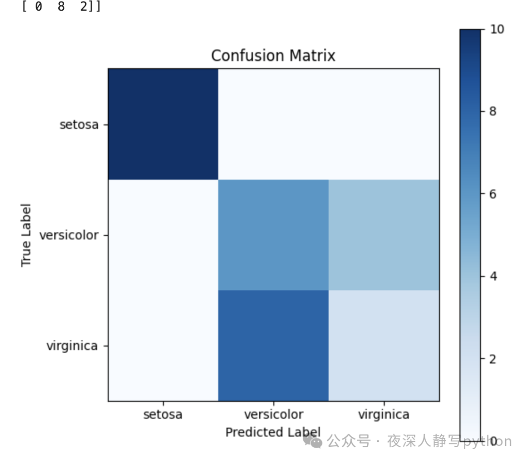
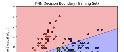
Visualization of decision boundary
def plot_decision_boundary(X, y, model, scaler, title):
    h = 0.02  # Grid step size
    x_min, x_max = X[:, 0].min() - 1, X[:, 0].max() + 1
    y_min, y_max = X[:, 1].min() - 1, X[:, 1].max() + 1

    xx, yy = np.meshgrid(np.arange(x_min, x_max, h), np.arange(y_min, y_max, h))

    # Construct grid points and transform them to standardized features consistent with training data
    grid_points = np.c_[xx.ravel(), yy.ravel()]
    grid_points_scaled = scaler.transform(grid_points)

    # Predict all grid points
    Z = model.predict(grid_points_scaled)

    # Ensure output shape matches the grid
    Z = Z.reshape(xx.shape)

    # Draw the decision boundary
    plt.contourf(xx, yy, Z, alpha=0.3, cmap=ListedColormap(['red', 'green', 'blue']))
    scatter = plt.scatter(X[:, 0], X[:, 1], c=y, edgecolors='k', cmap=ListedColormap(['red', 'green', 'blue']))
    plt.xlabel('Feature 1 (sepal length)')
    plt.ylabel('Feature 2 (sepal width)')
    plt.title(title)
    plt.show()

# Draw the decision boundary for the training set
plot_decision_boundary(X_train, y_train, knn, scaler, "KNN Decision Boundary (Training Set)")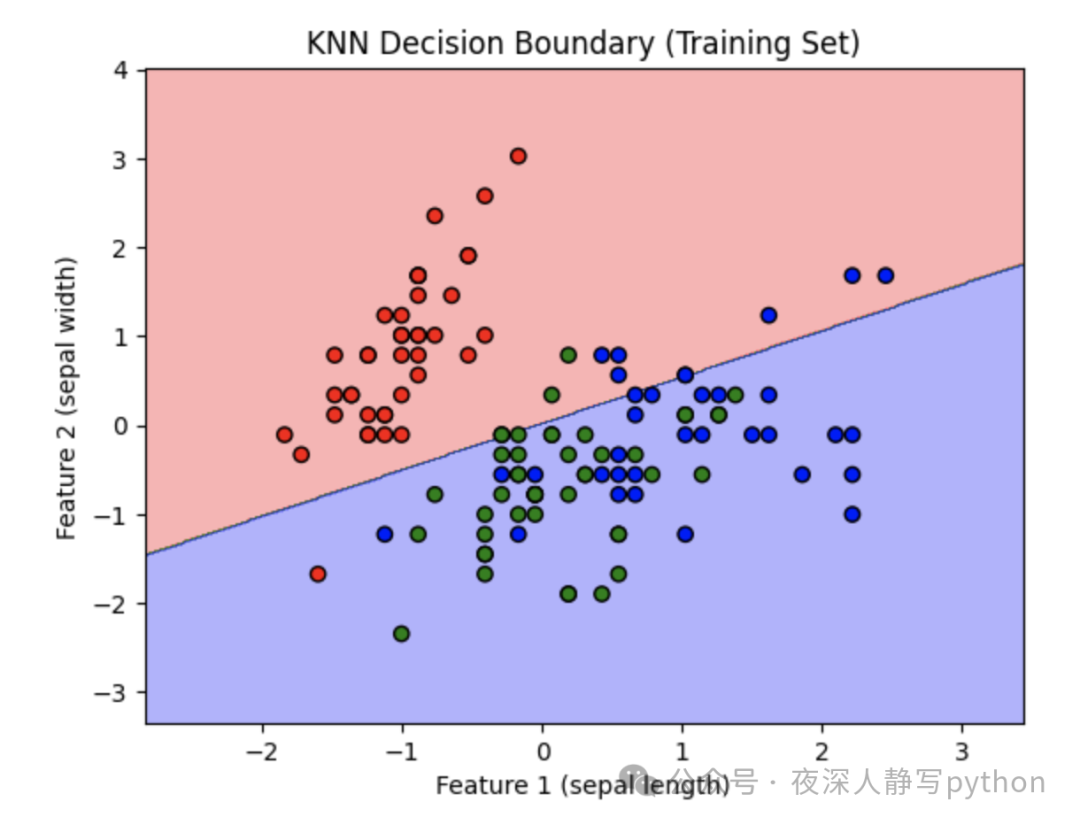
Finally
That’s all for today’s sharing. If you find it useful, please like and share it.