The K-Nearest Neighbors (KNN) model is a simple and effective machine learning algorithm mainly used for classification and regression tasks. The basic idea of KNN is that the class or value of a sample depends on the classes or values of its k nearest neighbors. Specifically, KNN predicts the class or value of a point by calculating the distances to all points in the training dataset, selecting the k nearest points as neighbors, and then using the classes or values of these neighbors to make the prediction.
Working Principle of KNN Model
The workflow of the KNN algorithm is as follows:
Distance Measurement: KNN uses distance measures (such as Euclidean distance, Manhattan distance, etc.) to determine the similarity between data points. The most common distance measure is Euclidean distance.
Choosing K Value: K is a hyperparameter that represents the number of nearest neighbors considered in making decisions. The choice of K significantly impacts the model’s performance, and the optimal K value is generally determined using methods like grid search.
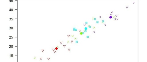
Decision: For classification tasks, the KNN algorithm predicts the class of new samples by majority voting; for regression tasks, it calculates the average of the target values of the K nearest neighbors as the target value for the new sample.
Advantages and Disadvantages of KNN Model
Advantages:
Simple and Easy to Understand: The concept of the KNN algorithm is straightforward, making it easy to understand and implement.
No Training Phase Needed: KNN does not have an explicit training phase; it only needs to store the training dataset, which allows for faster modeling training speed under the same conditions of dataset size and feature number.
Suitable for Small Datasets: KNN typically performs well on small datasets.
Disadvantages:
High Computational Cost: For large-scale datasets, calculating the distance from each test sample to all samples in the training set can be very time-consuming.
High Memory Consumption: It requires storing all training data for distance calculations.
Sensitive to Outliers: The choice of neighbors is very sensitive to outliers, which can lead to model instability.
Application Scenarios and Real Cases
The KNN algorithm has a wide range of applications in practice, such as:
Text Classification: Used to classify text data into different categories.
Image Recognition: Identifying image content by comparing image features.
Recommendation Systems: Recommending related products or content based on users’ purchase or browsing history.
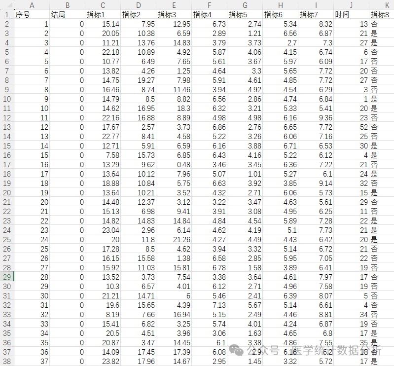
Today, we will demonstrate the basic operations of the K-Nearest Neighbors (KNN) model in Python using a familiar example dataset, as well as the evaluation using ROC curves and confusion matrices.
# Load packages (openpyxl, pandas, etc.)
# Use pandas to read the example data xlsx file
import openpyxl
import pandas as pd
import matplotlib.pyplot as plt
import sklearn
from sklearn.model_selection import train_test_split
from sklearn.neighbors import KNeighborsClassifier
# Load dataset
dataknn = pd.read_excel(r’C:\Users\L\Desktop\example_data.xlsx’)
# View the first few rows of data
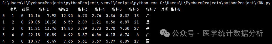
print(dataknn.head())
# Separate features and target variable
X = dataknn[[‘Feature1’, ‘Feature2’, ‘Feature3′,’Feature4′,’Feature5′,’Feature6’]]
y = dataknn[‘Outcome’]
# Split into training and test sets
X_train, X_test, y_train, y_test = train_test_split(X, y, test_size=0.3, random_state=42)
# Create and train the model
knn = KNeighborsClassifier(n_neighbors=5)
knn.fit(X_train, y_train)
# Predict and evaluate the model
predictions = knn.predict(X_test)
accuracy = knn.score(X_test, y_test)
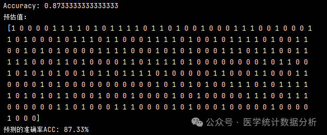
print(f”Accuracy: {accuracy}”)
print(“Predicted values:
“, predictions)
acc = sum(predictions == y_test) / predictions.shape[0]
print(“Predicted accuracy ACC: %.2f%%” % (acc*100))
# Confusion matrix evaluation of the model
# Import third-party module
from sklearn import metrics
# Confusion matrix
print(“Confusion matrix four-grid table output as follows:”)
print(metrics.confusion_matrix(y_test, predictions, labels = [0, 1]))
Accuracy = metrics._scorer.accuracy_score(y_test, predictions)
Sensitivity = metrics._scorer.recall_score(y_test, predictions)
Specificity = metrics._scorer.recall_score(y_test, predictions, pos_label=0)
print(“KNN model confusion matrix evaluation results as follows:”)
print(‘Model accuracy is %.2f%%’ % (Accuracy*100))
print(‘Positive coverage rate is %.2f%%’ % (Sensitivity*100))
print(‘Negative coverage rate is %.2f%%’ % (Specificity*100))

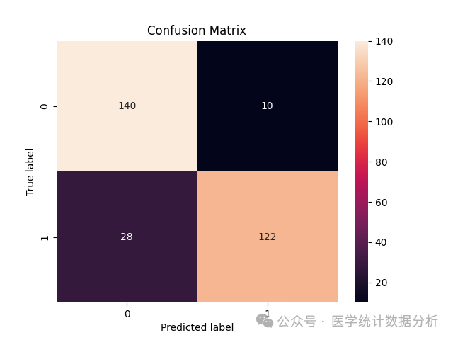
# Use Seaborn’s heatmap to draw the confusion matrix
import matplotlib.pyplot as plt
from sklearn.metrics import confusion_matrix
import seaborn as sns
sns.heatmap(metrics.confusion_matrix(y_test, predictions), annot=True, fmt=’d’)
plt.title(‘Confusion Matrix’)
plt.xlabel(‘Predicted label’)
plt.ylabel(‘True label’)
plt.show()
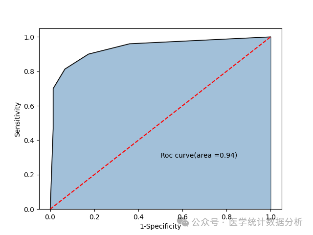
# Prepare for ROC curve plotting and calculation
# y_score is the model’s predicted probability of positive cases
y_score = knn.predict_proba(X_test)[:,1]
# Calculate combinations of fpr and tpr at different thresholds, where fpr represents 1-Specificity, and tpr represents sensitivity
fpr, tpr, threshold = metrics.roc_curve(y_test, y_score)
# Calculate the AUC value
roc_auc = metrics.auc(fpr, tpr)
print(“KNN model predicted test set ROC curve AUC:”, roc_auc)
KNN model predicted test set ROC curve AUC: 0.9356444444444444
# Plot ROC curve
import matplotlib.pyplot as plt
import seaborn as sns
# Draw area chart
plt.stackplot(fpr, tpr, color=’steelblue’, alpha = 0.5, edgecolor = ‘black’)
# Add marginal line
plt.plot(fpr, tpr, color=’black’, lw = 1)
# Add diagonal line
plt.plot([0,1],[0,1], color =’red’, linestyle =’–‘)
# Add text information
plt.text(0.5,0.3, ‘Roc curve(area =%.2f)’ % roc_auc)
# Add axis labels
plt.xlabel(‘1-Specificity’)
plt.ylabel(‘Sensitivity’)
# Show the figure
plt.show()
Sharing experiences in medical statistical data analysis using SPSS, R, Python, ArcGis, Geoda, GraphPad, and data analysis chart creation. Accepting data analysis, paper revisions, medical statistics, spatial analysis, and questionnaire analysis services. If you have submission and data analysis outsourcing needs, please contact me directly, thank you!