MLNLP Community is a well-known machine learning and natural language processing community in China and abroad, covering NLP master’s and PhD students, university teachers, and corporate researchers.

Community Vision is to promote communication and progress between the academic and industrial circles of natural language processing and machine learning, especially for beginners.

Reprinted from | Zhihu

Author丨tian-feng

1. Introduction (Can Be Skipped)

Hello, everyone, I am Tian-Feng. Today I will introduce some principles of stable diffusion. The content is easy to understand, as I usually play with AI painting, so I wrote this article to explain its principles. It took me quite a long time to write this article, and if you find it useful, I hope you can like it. Thank you.

Stable diffusion, as the open-source image generation model from Stability-AI, is no less significant than ChatGPT. Its development momentum is on par with midjourney, and with the support of numerous plugins, its launch has also been greatly enhanced. Of course, the methods are slightly more complex than midjourney.

As for why it is open-source, the founder said: The reason I do this is that I believe it is part of a shared narrative; some people need to publicly display what has happened. I want to emphasize again that this should be assumed to be open-source by default. Because value does not exist in any proprietary model or data, we will build auditable open-source models, even if they contain licensed data. Without further ado, let’s get started.

2. Stable Diffusion

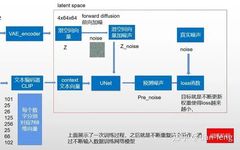
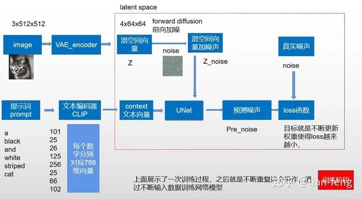
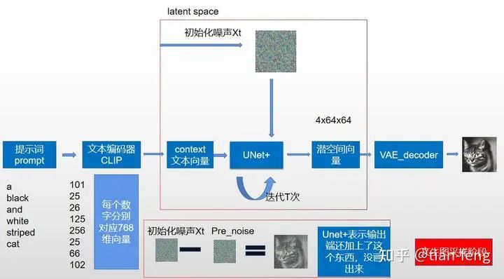
For the image in the original paper above, it may be difficult for everyone to understand, but that’s okay; I will break down the image into individual modules for interpretation and then combine them, and I believe you will understand what each step of the image does.

First, I will draw a simplified model diagram corresponding to the original image for easier understanding. Let’s start from the training phase. You might notice that the VAE decoder is missing; this is because our training process is completed in latent space. We will discuss the decoder in the second phase, the sampling stage. The stablediffusion webui we use for drawing is usually in the sampling phase. As for the training phase, most ordinary people cannot complete it; the training time required should be measurable in GPU years (a single V100 GPU takes a year). If you have 100 cards, you should be able to complete it in a month. As for ChatGPT, the electricity cost is tens of millions of dollars, with thousands of GPU clusters. It feels like AI is now all about computing power. I digress, come back.

Understanding Stable Diffusion Principles in Simple Terms

1. CLIP

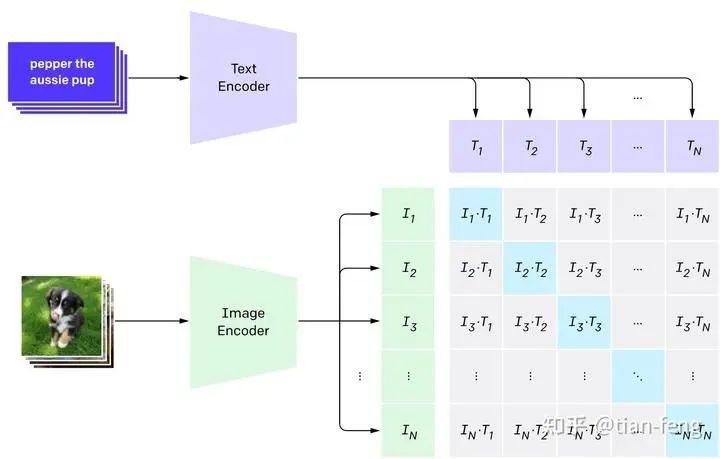
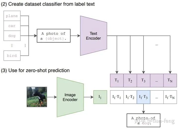
Let’s start with the prompt. We input a prompt a black and white striped cat, and CLIP will correspond the text to a vocabulary list, with each word and punctuation mark corresponding to a number. We call each word a token. Previously, stable diffusion had a limit of 75 words (which is no longer the case), meaning 75 tokens. You may notice that 6 words correspond to 8 tokens because it also includes a start token and an end token. Each number corresponds to a 768-dimensional vector, which you can think of as an ID card for each word, and words with very similar meanings correspond to similar 768-dimensional vectors. Through CLIP, we obtain a (8,768) text vector corresponding to the image.

The stable diffusion uses OpenAI’s pre-trained CLIP model, which means we are using a model that has already been trained. How was CLIP trained? How does it correspond images with text information? (The following expansion can be viewed or skipped; it does not affect understanding; just know that it is used to convert prompts into corresponding image-generating text vectors.)

CLIP requires data consisting of images and their titles, with the dataset containing about 400 million images and descriptions. It should have been obtained directly through web scraping, with image information directly used as labels. The training process is as follows:

CLIP is a combination of an image encoder and a text encoder, using two encoders to encode the data separately. Then, cosine distance is used to compare the result embeddings. At the beginning of training, even if the text description matches the image, their similarity is definitely low.

As the model continues to update, in subsequent stages, the embeddings obtained from the image and text encoders will become increasingly similar. This process is repeated throughout the dataset, using a large batch size encoder, ultimately generating an embedding vector where the image of a dog and the sentence “an image of a dog” are similar.

When given some prompt text, the similarity is calculated for each prompt, and the one with the highest probability is selected.

2. Diffusion Model

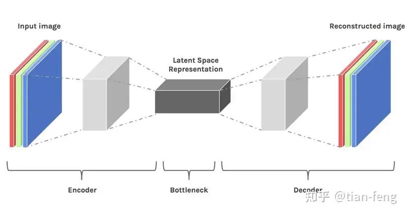
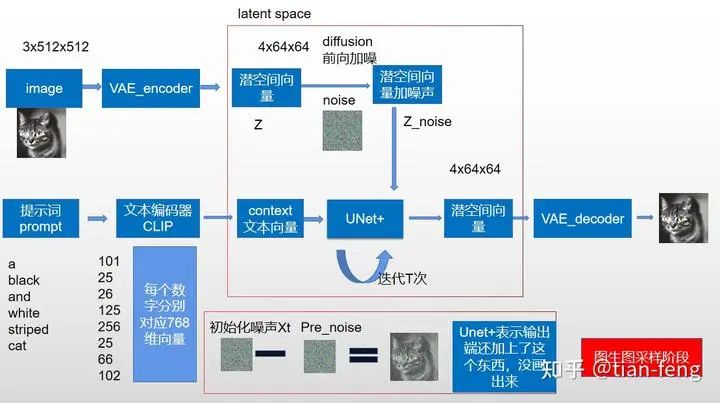
Now that we have the input for the UNet, we still need an input noise image. If we input a 3x512x512 cat image, we do not directly process the cat image; instead, we compress the 512×512 image from pixel space to latent space (4x64x64) through the VAE encoder, reducing the data volume by nearly 64 times.

Latent space is simply a representation of compressed data. Compression refers to the process of encoding information using fewer digits than the original representation. Dimensionality reduction may lose some information; however, in some cases, reducing dimensions is not a bad thing. By filtering out less important information, we can retain the most important information.

After obtaining the latent space vector, we now enter the diffusion model. The secret behind why the image can be restored after being noised lies in the formula. Here, I will explain the theory using the DDPM paper. Of course, there are also improved versions like DDIM, etc., which you can refer to if you’re interested.

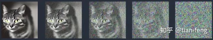
Forward Diffusion

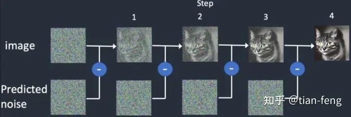
First is the forward diffusion, which is the noise-adding process, ultimately turning into pure noise.
At each moment, Gaussian noise must be added, and the next moment is obtained by adding noise to the previous moment.

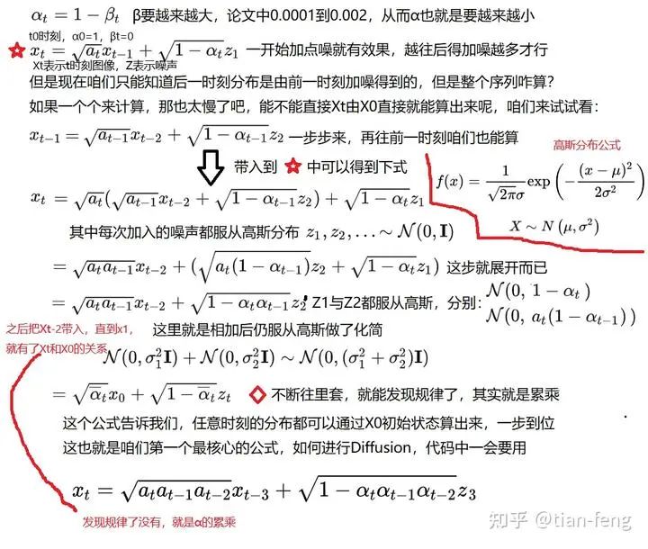
So, do we need to obtain noise from the previous step every time we add noise? Can we obtain the noise image at any step we want? The answer is YES. The reason is: in our training process, adding noise to the image is random. If we randomly get noise for 100 steps (assuming the time steps are set to 200), if we want to add noise from the first step to get the second step, it would be too time-consuming to repeat this. In fact, the added noise follows a pattern. Our current goal is to derive any moment’s noise image from the original image X0 without having to get the desired noise image step by step.

I will explain the above. I have labeled everything clearly.

First, the range of αt is 0.9999-0.998.

Second, the noise added to the image follows a Gaussian distribution, meaning the noise added to the latent space vector has a mean of 0 and a variance of 1. By bringing Xt-1 into Xt, why can the two terms be combined? Because Z1 and Z2 both follow a Gaussian distribution, their sum Z2′ also follows a Gaussian distribution, and their variances sum to a new variance. Therefore, we sum their respective variances (the square root is the standard deviation). If you cannot understand, you can treat it as a theorem. To elaborate, for Z–>a+bZ, Z’s Gaussian distribution changes from (0,σ)>(a,bσ). Now we have obtained the relationship between Xt and Xt-2.

Third, if you bring Xt-2 in, you can get the relationship with Xt-3, and by finding the pattern, you can get the cumulative product of α, ultimately obtaining the relationship between Xt and X0. Now we can directly obtain the noise image at any moment based on this formula.

Fourth, because the initialized noise for the image is random, let’s assume the time steps you set (timesteps) are 200, meaning dividing the interval of 0.9999-0.998 into 200 parts, representing the α value at each moment. According to the formula of Xt and X0, because α is cumulative (the smaller it is), it can be seen that as you go further back, the noise increases faster, roughly from 1-0.13. At time 0, α is 1, representing the image itself, and at time 200, the image has roughly α of 0.13, meaning noise occupies 0.87. Since this is cumulative, the noise increases, and it is not an average process.

Fifth, to add, the Reparameterization Trick states if X(u,σ2), then X can be expressed as X=μ+σZ, where Z~Ν(0,1). This is the reparameterization trick.

The reparameterization trick allows sampling from a distribution with parameters. If sampling is done directly (the sampling action is discrete and non-differentiable), there is no gradient information, meaning that during backpropagation, the parameter gradients will not be updated. The reparameterization trick ensures that we can sample while retaining gradient information.

Reverse Diffusion

After the forward diffusion is completed, the next step is reverse diffusion, which may be more challenging than the previous one. How to obtain the original image step by step from a noisy image is the key.

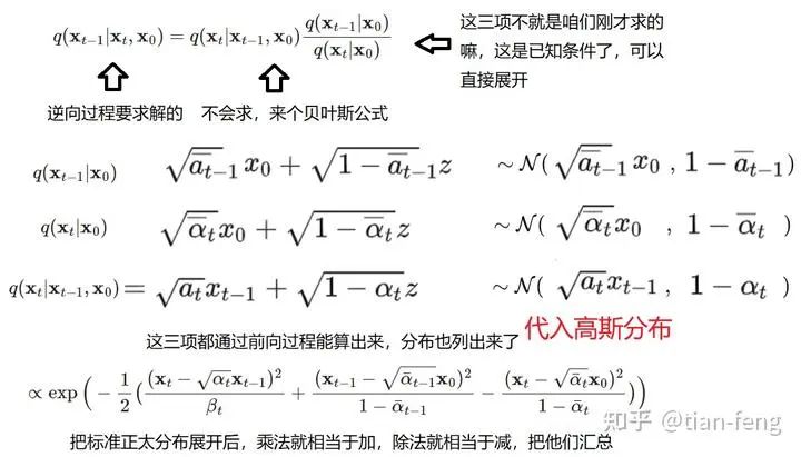
Starting the reverse process, our goal is to obtain the noise image Xt to get the noise-free X0. We first seek Xt-1 from Xt, where we initially assume X0 is known (ignoring why we assume it is known). Later, we will replace it. As for how to replace it, isn’t the relationship between Xt and X0 known from forward diffusion? Now we know Xt, we can express X0 in terms of Xt, but there is still an unknown Z noise. This is where UNet comes into play, as it needs to predict the noise.
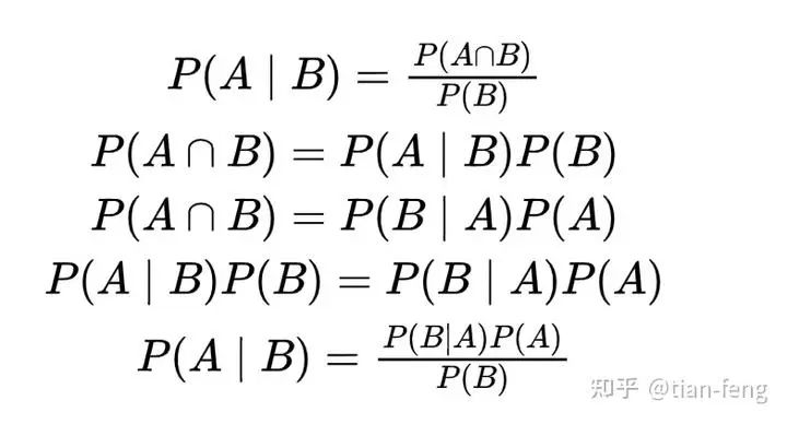
Here we utilize Bayes’ theorem (which is conditional probability). We rely on the results from Bayes’ theorem; I previously wrote a document (https://tianfeng.space/279.html).

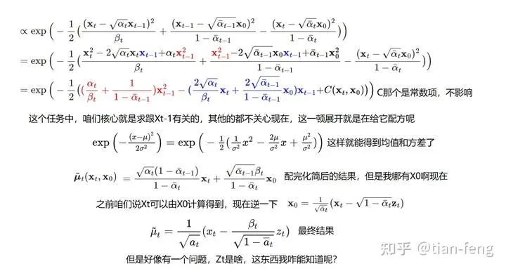
We seek Xt-1 from Xt, and in reverse we do not know how to seek it, but if we know X0, we can derive the other terms.

Starting the interpretation, since these three terms all follow Gaussian distributions, bringing them into the Gaussian distribution (also known as the normal distribution), why does their multiplication equal addition? Because e2 * e3 = e2+3, which can be understood (it belongs to exp, i.e., exponentiation). Now we have obtained an overall equation, and we will continue to simplify.

First, we expand the square, leaving Xt-1 as the only unknown. We format it as AX2+BX+C. Don’t forget, even if added, it still follows a Gaussian distribution. Now we format the original Gaussian distribution formula similarly, with the red part being the inverse of the variance. By multiplying the blue part by the variance divided by 2, we obtain the mean μ (the simplification result is shown below; if you are interested, you can simplify it yourself). Returning to X0, previously assuming X0 is known, we now express it in terms of Xt (known), substituting μ, leaving only Zt as the unknown.

Zt is actually the noise we want to estimate at each moment – here we use the UNet model for prediction. The model’s input parameters are three: the current distribution Xt, the time step t, and the previous text vector, and it outputs the predicted noise. This is the whole process.

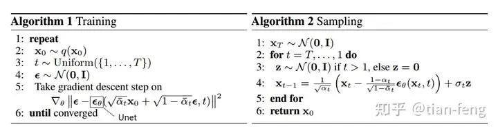
The above Algorithm 1 is the training process.

The second step generally refers to taking data, usually a class of images like cats or dogs, or images of a certain style. You cannot mix various images randomly, or the model will not learn.

The third step states that each image is randomly assigned a moment of noise (as mentioned above).

The fourth step states that the noise follows a Gaussian distribution.

The fifth step calculates the loss between the real noise and the predicted noise (DDPM input does not have a text vector, so it is not written; you can understand it as adding an input), updating parameters until the output noise is very close to the real noise, completing the training of the UNet model.

Next, we arrive at Algorithm 2, the sampling process.

It simply states that Xt follows a Gaussian distribution.
Perform T times to sequentially seek Xt-1 to X0, which are T moments.
Xt-1 is the formula derived from our reverse diffusion, Xt-1=μ+σZ, where the mean and variance are known, and the only unknown noise Z is predicted by the UNet model.

Sampling Diagram

For ease of understanding, I will separately illustrate text-to-image and image-to-image. If you are using stable diffusion webui to draw, you will find it very familiar. If it’s text-to-image, it initializes a noise and samples directly.
Image-to-image, on the other hand, adds noise to an existing image, where the noise weight is controlled by the user. Isn’t there a redraw amplitude in the webui interface? That’s it.
The number of iterations is the sampling steps in our webui interface.
The random seed is a noise image obtained initially, so if you want to replicate the same image, the seed must remain consistent.

Stage Summary

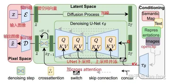
Now let’s look at this diagram again. Besides UNet, which I haven’t explained (I will introduce separately below), isn’t it much simpler? The far left is the encoder-decoder in pixel space, the far right is CLIP converting text into text vectors, the upper middle is noise addition, and the lower part is UNet predicting noise, continuously sampling to obtain the output image. This is the sampling diagram from the original paper; the training process is not illustrated.

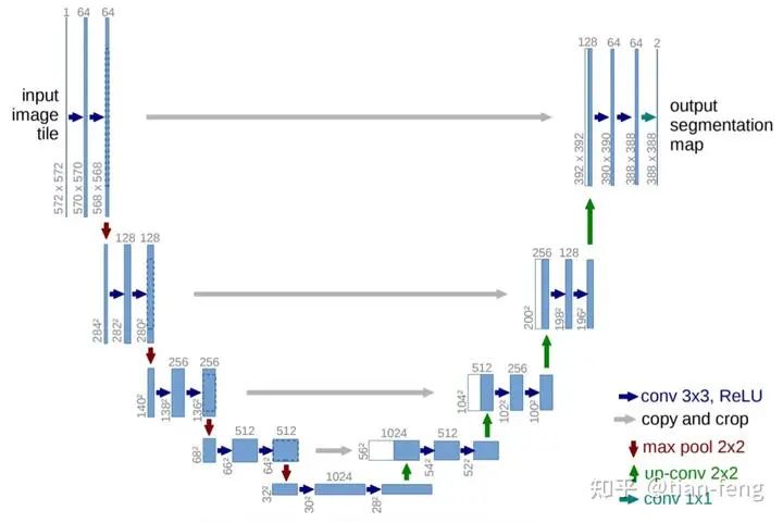
3. UNet Model

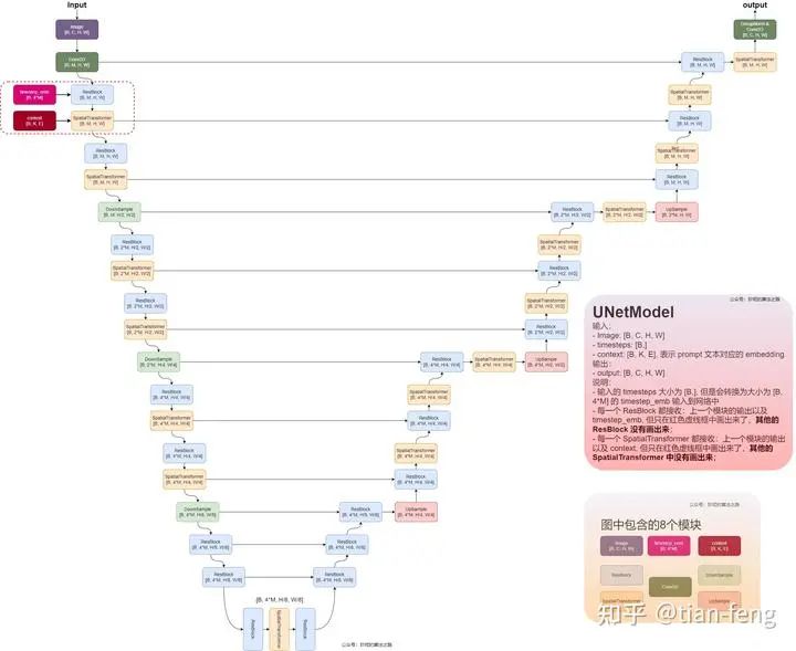
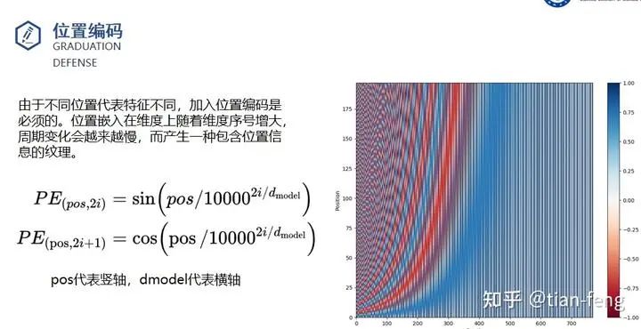
The UNet model is something many of you may know to some extent, involving multi-scale feature fusion, like FPN image pyramid, PAN, which share similar ideas. Typically, ResNet is used as the backbone (downsampling) to serve as the encoder, allowing us to obtain multiple scale feature maps, and during the upsampling process, we concatenate the feature maps obtained from downsampling. This is a standard UNet.

So, what is different about the UNet used in stable diffusion? Here’s a diagram I found. I admire this lady’s patience, so I borrowed her diagram.

I will explain the ResBlock module and SpatialTransformer module. The inputs are timestep_embedding, context, and input, which are the three inputs: time step, text vector, and noisy image. You can understand the time step as position encoding in transformers, used in natural language processing to inform the model about the positional information of each word in a sentence. Different positions can have significantly different meanings, and here, adding time step information can be understood as informing the model about the noise addition at which step (of course, this is my interpretation).

Timestep_embedding uses sine and cosine encoding

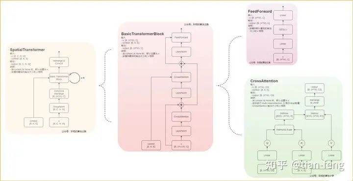
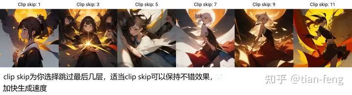
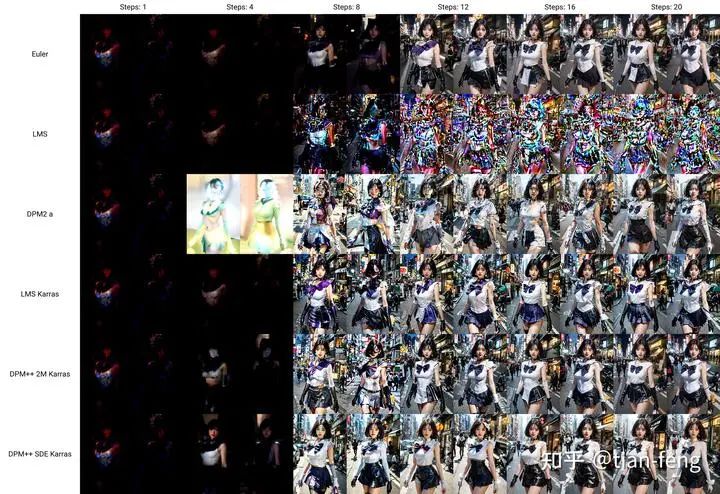
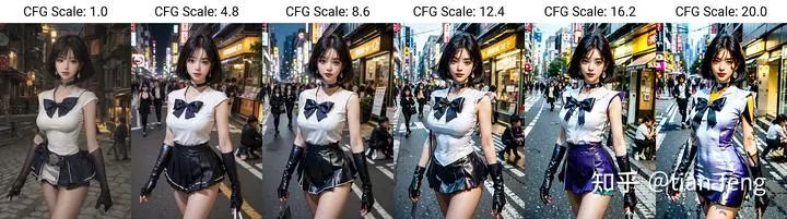
The ResBlock module takes the time encoding and the convolved image output and adds them together. This is its function; I won’t go into the details, as convolution and fully connected layers are quite simple.

The SpatialTransformer module takes the text vector and the output from the previous ResBlock.

It mainly discusses cross attention; the rest involves some dimensional transformations, convolution operations, and various normalizations such as Group Norm and Layer Norm.

Using cross attention, the features of the latent space are fused with the features of another modal sequence (text vector) and added to the reverse process of the diffusion model. Through UNet, the noise to be reduced at each step is predicted, calculating gradients using the loss function between the ground truth noise and the predicted noise.

Looking at the diagram in the lower right corner, you can see that Q represents the features of the latent space, while KV are the text vectors, which are both connected through two fully connected layers. The remaining operations are standard transformer operations. After multiplying Q and K, applying softmax gives a score, which is then multiplied by V, transforming the dimensions for output. You can think of the transformer as a feature extractor that highlights important information (just for understanding). That’s about it; the subsequent operations are quite similar, ultimately outputting the predicted noise.

Here, you should be familiar with transformers and know what self-attention and cross-attention are; if you don’t understand, look for an article to read, as it’s not something that can be simply explained.

That’s all, goodbye, displaying some comparison images from webui.

3. Stable Diffusion WebUI Extensions

Parameters clip

Technical Group Invitation

Understanding Stable Diffusion Principles in Simple Terms

△ Long press to add the assistant

Scan the QR code to add the assistant on WeChat

Please note: Name – School/Company – Research Direction

(For example: Xiao Zhang – Harbin Institute of Technology – Dialogue System)

to apply for joining the Natural Language Processing/Pytorch technical group