
0
Introduction
0
Introduction
Recently, AI drawing has become very popular, and one of the core technologies behind it is the Diffusion Model. Although fully understanding the Diffusion Model and its complex formula derivation requires a solid foundation in mathematics, this does not prevent us from grasping its principles. The following will explain what the Diffusion Model is from the author’s understanding.
1
What is the Diffusion Model
1
What is the Diffusion Model
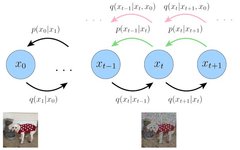
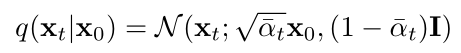
Forward Diffusion Process
The Diffusion Model first defines a forward diffusion process that includes a total of <span>T</span> time steps, as shown in the figure below:
The leftmost blue circle <span>x0</span> represents the real natural image, corresponding to the dog image below.
The rightmost blue circle <span>xT</span> represents pure Gaussian noise, corresponding to the noise image below.
The middle blue circle <span>xt</span> represents the noisy <span>x0</span>, corresponding to the noisy dog image below.
The arrow below <span>q(xt|xt-1)</span> represents a Gaussian distribution with the previous state <span>xt-1</span> as the mean, from which <span>xt</span> is sampled.
The so-called forward diffusion process can be understood as a Markov chain (see reference <span>[7]</span>), which gradually adds Gaussian noise to a real image until it eventually becomes a pure Gaussian noise image.
So how exactly is noise added? The formula is as follows:
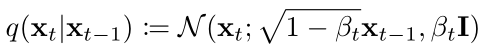
Each time step’s <span>xt</span> is sampled from a Gaussian distribution with <span>1-βt</span> multiplied by the square root of <span>xt-1</span> as the mean, and <span>βt</span> as the variance.
Where <span>βt, t ∈ [1, T]</span> are a series of fixed values generated by a formula.
In reference <span>[2]</span>, set <span>T=1000, β1=0.0001, βT=0.02</span>, and generate all <span>βt</span> values with one line of code:
# https://pytorch.org/docs/stable/generated/torch.linspace.html
betas = torch.linspace(start=0.0001, end=0.02, steps=1000)
When sampling to obtain <span>xt</span>, it is not sampled directly from the Gaussian distribution <span>q(xt|xt-1)</span>, but uses a reparameterization trick (see reference <span>[4]</span> page 5).
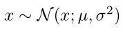
In simple terms, if you want to sample from a Gaussian distribution with any mean <span>μ</span> and variance <span>σ^2</span>, you can first sample from a standard Gaussian distribution (mean 0, variance 1) to get <span>ε</span>,
Then <span>μ + σ·ε</span> is equivalent to the result of sampling from any Gaussian distribution. The formula is as follows:
Next, let’s look at how to sample to obtain the noise image <span>xt</span>,

First, sample from a standard Gaussian distribution, then multiply by the standard deviation and add the mean, pseudo-code is as follows:
# https://pytorch.org/docs/stable/generated/torch.randn_like.html
betas = torch.linspace(start=0.0001, end=0.02, steps=1000)
noise = torch.randn_like(x_0)
ext = sqrt(1-betas[t]) * xt-1 + sqrt(betas[t]) * noise
Then the forward diffusion process has another property, which is that you can directly sample from <span>x0</span> to get the noise image at any intermediate time step <span>xt</span>, the formula is as follows:

Where <span>αt</span> represents:
The specific derivation can be found in reference <span>[4]</span> page 11, pseudo-code is as follows:
betas = torch.linspace(start=0.0001, end=0.02, steps=1000)
alphas = 1 - betas
# cumprod is equivalent to calculating a prefix product for each time step t
# https://pytorch.org/docs/stable/generated/torch.cumprod.html
alphas_cum = torch.cumprod(alphas, 0)
alphas_cum_s = torch.sqrt(alphas_cum)
alphas_cum_sm = torch.sqrt(1 - alphas_cum)

# Apply the reparameterization trick to sample xt
noise = torch.randn_like(x_0)
ext = alphas_cum_s[t] * x_0 + alphas_cum_sm[t] * noise
Through the above explanation, readers should have a clear understanding of the forward diffusion process of the Diffusion Model.
But our goal is to generate images, right?
Now we have only obtained a noise image from the real image in the dataset, so how do we generate images specifically?
Reverse Diffusion Process

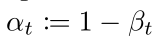
The reverse diffusion process <span>q(xt-1|xt, x0)</span><span> (see pink arrow) is the posterior probability distribution of the forward diffusion process </span><code><span>q(xt|xt-1)</span>.
In contrast to the forward process, it starts from the pure Gaussian noise image on the right and gradually samples to obtain the real image <span>x0</span>.
The posterior probability <span>q(xt-1|xt, x0) </span> can be derived based on Bayes’ theorem (the derivation process can be found in reference <span>[4]</span> page 12):
It is also a Gaussian distribution.
Its variance can be seen as a constant, and the variance value for all time steps can be calculated in advance:

The calculation pseudo-code is as follows:
betas = torch.linspace(start=0.0001, end=0.02, steps=1000)
alphas = 1 - betas
alphas_cum = torch.cumprod(alphas, 0)
alphas_cum_prev = torch.cat((torch.tensor([1.0]), alphas_cum[:-1]), 0)
posterior_variance = betas * (1 - alphas_cum_prev) / (1 - alphas_cum)
Next, let’s look at the calculation of the mean,
For the reverse diffusion process, when sampling to generate <span>xt-1</span>, <span>xt</span> is known, while the other coefficients are constants that can be calculated in advance.
However, the problem now is that when generating images through the reverse process, we do not know <span>x0</span>, because it is the target image to be generated.
It seems to have become a chicken-and-egg problem, so what should we do?
Diffusion Model Training Objective
When a probability distribution <span>q</span> is difficult to solve, we can change our approach (see reference <span>[5,6]</span>).
By artificially constructing a new distribution <span>p</span>, the goal is to minimize the difference between distributions <span>p</span> and <span>q</span>.
By continuously modifying the parameters of <span>p</span> to minimize the difference, when <span>p</span> and <span>q</span> are sufficiently similar, it can replace <span>q</span>.
Returning to the reverse diffusion process, since the posterior distribution <span>q(xt-1|xt, x0)</span> cannot be solved directly.
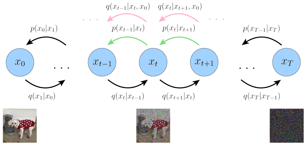
We construct a Gaussian distribution <span>p(xt-1|xt)</span><span> (see green arrow) to make its variance consistent with the posterior distribution </span><code><span>q(xt-1|xt, x0)</span>:
Its mean is set to:
The difference from <span>q(xt-1|xt, x0)</span><span> is that </span><code><span>x0</span> is replaced by <span>xθ(xt, t)</span>, predicted by a deep learning model, with model input being the noisy image <span>xt</span> and time step <span>t</span>.
Then minimize the difference between distributions <span>p(xt-1|xt)</span> and <span>q(xt-1|xt, x0)</span>, transforming it into optimizing the following objective function (the derivation process can be found in reference <span>[4]</span> page 13):
However, if we let the model predict directly from <span>xt</span> to <span>x0</span>, the fitting difficulty is too high, so we continue to change our approach.
In the previous introduction of the forward diffusion process, it was mentioned that <span>xt</span> can be directly obtained from <span>x0</span>:
Transforming the above formula yields:
Substituting into the mean expression of <span>q(xt-1|xt, x0) </span> gives (the derivation process can be found in reference <span>[4]</span> page 15):
Observing the transformed expression above, we find that the mean of the posterior probability <span>q(xt-1|xt, x0) </span> only relates to <span>xt</span> and the noise added during the forward diffusion process at time step <span>t</span>.
So we also modify the mean of the constructed distribution <span>p(xt-1|xt)</span>:
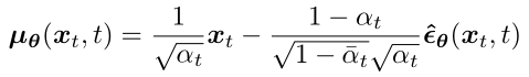
We change the model to predict the Gaussian noise <span>ε</span> added at the forward time step <span>t</span>, with model input being <span>xt</span> and time step <span>t</span>:

Then the optimized objective function becomes (the derivation process can be found in reference <span>[4]</span> page 15):
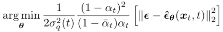
Then the algorithm description of the training process is as follows, the coefficients in front of the final objective function are removed because they are constants:
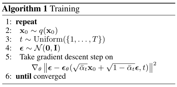
It can be seen that although the derivation process is complex, the training process is quite simple.
First, each iteration involves taking a real image <span>x0</span> from the dataset and sampling a time step <span>t</span> from a uniform distribution,
Then sample noise <span>ε</span> from the standard Gaussian distribution and calculate <span>xt</span> according to the formula.
Next, input <span>xt</span> and <span>t</span> into the model to let it output a fit for the predicted noise <span>ε</span>, and update the model through gradient descent until convergence.
The deep learning model used is similar to the structure of <span>UNet</span> (see reference <span>[2]</span> Appendix B).
The pseudo-code for the training process is as follows:
betas = torch.linspace(start=0.0001, end=0.02, steps=1000)
alphas = 1 - betas
alphas_cum = torch.cumprod(alphas, 0)
alphas_cum_s = torch.sqrt(alphas_cum)
alphas_cum_sm = torch.sqrt(1 - alphas_cum)

def diffusion_loss(model, x0, t, noise):
    # Calculate xt according to the formula
    xt = alphas_cum_s[t] * x0 + alphas_cum_sm[t] * noise
    # Model predicts noise
    predicted_noise = model(xt, t)
    # Calculate Loss
    return mse_loss(predicted_noise, noise)

for i in len(data_loader):
    # Read a batch of real images from the dataset
    x0 = next(data_loader)
    # Sample time step
    t = torch.randint(0, 1000, (batch_size,))
    # Generate Gaussian noise
    noise = torch.randn_like(x_0)
    loss = diffusion_loss(model, x0, t, noise)
    optimizer.zero_grad()
    loss.backward()
    optimizer.step()
Diffusion Model Image Generation Process
After the model is trained, during the real inference phase, images must be generated step by step starting from time step <span>T</span>, the algorithm description is as follows:
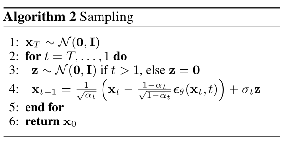
Initially, generate noise from the standard Gaussian distribution, then at each time step <span>t</span>, input the previously generated image <span>xt</span> into the model to predict the noise. Next, sample noise from the standard Gaussian distribution, and calculate <span>xt-1</span> based on the reparameterization trick and the posterior probability mean and variance formulas until time step <span>1</span> is reached.
2
Improving the Diffusion Model
2
Improving the Diffusion Model
The article <span>[3]</span> proposes some improvements to the Diffusion Model.
Improvement of Variance βt
It was mentioned earlier that the generation of <span>βt</span> divides a given range uniformly into <span>T</span> parts, with each time step corresponding to a certain point:
betas = torch.linspace(start=0.0001, end=0.02, steps=1000)
Then the article <span>[3]</span> observes through experiments that using this method to generate variance <span>βt</span> leads to a problem where too much noise is added at the later time steps during forward diffusion.
This results in the fact that during the later time steps in the forward process, there is not much contribution during reverse generation sampling, and skipping them would not have a significant impact on the generation results.
The paper <span>[3]</span> then proposes a new generation strategy for <span>βt</span>, with a comparison to the original strategy during forward diffusion shown in the figure below:
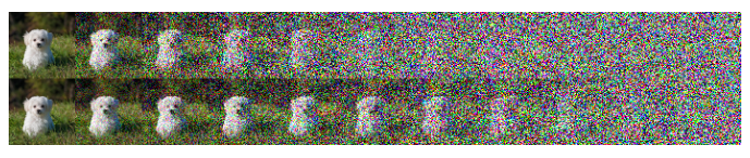
The first row is the original generation strategy, and it can be seen that it has already become pure Gaussian noise before reaching the final time step,
While in the second row, the improved strategy adds noise more slowly, which seems more reasonable.
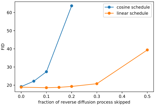
Experimental results show that for images from the imagenet dataset <span>64x64</span>, the original strategy during reverse diffusion shows that even skipping the first 20% of time steps does not significantly affect the metrics.
Now let’s look at the new proposed strategy formula:
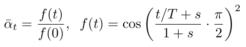
Where <span>s</span> is set to <span>0.008</span> and the maximum value of <span>βt</span> is limited to <span>0.999</span>, the pseudo-code is as follows:
T = 1000
s = 8e-3
ts = torch.arange(T + 1, dtype=torch.float64) / T + s
alphas = ts / (1 + s) * math.pi / 2
alphas = torch.cos(alphas).pow(2)
alphas = alphas / alphas[0]
betas = 1 - alphas[1:] / alphas[:-1]
betas = betas.clamp(max=0.999)
Improvement of Number of Time Steps in the Generation Process
Originally, the model is trained under the assumption of <span>T</span> time steps, and during image generation, it must also traverse from <span>T</span> to <span>1</span>. The paper <span>[3]</span> proposes a method to reduce the number of generation steps without retraining, thus significantly improving generation speed.
This method simply describes that the original <span>T</span> time steps are now set to a smaller number of time steps <span>S</span>, mapping each time step <span>s</span> in the <span>S</span> time series to the steps in the <span>T</span> time series, the pseudo-code is as follows:
T = 1000
S = 100
start_idx = 0
all_steps = []
frac_stride = (T - 1) / (S - 1)
cur_idx = 0.0
s_timesteps = []
for _ in range(S):
    s_timesteps.append(start_idx + round(cur_idx))
    cur_idx += frac_stride
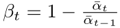
Next, calculate the new <span>β</span>, <span>St</span> is the computed <span>s_timesteps</span>:

The pseudo-code is as follows:
alphas = 1 - betas
alphas_cum = torch.cumprod(alphas, 0)
last_alpha_cum = 1.0
new_betas = []
# Iterate through the original alpha prefix product sequence
for i, alpha_cum in enumerate(alphas_cum):
    # When the index i in the original sequence T is in the new sequence S, calculate the new beta
    if i in s_timesteps:
        new_betas.append(1 - alpha_cum / last_alpha_cum)
        last_alpha_cum = alpha_cum
Let’s look at the experimental results:
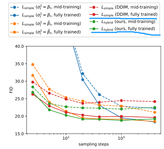
Focusing on the red and green solid lines of the blue line, it can be seen that reducing the sampling steps from <span>1000</span> to <span>100</span> does not significantly decrease the metrics.
References
-
[1] https://www.assemblyai.com/blog/diffusion-models-for-machine-learning-introduction/ -
[2] https://arxiv.org/pdf/2006.11239.pdf -
[3] https://arxiv.org/pdf/2102.09672.pdf -
[4] https://arxiv.org/pdf/2208.11970.pdf -
[5] https://www.zhihu.com/question/41765860/answer/1149453776 -
[6] https://www.zhihu.com/question/41765860/answer/331070683 -
[7] https://zh.wikipedia.org/wiki/%E9%A9%AC%E5%B0%94%E5%8F%AF%E5%A4%AB%E9%93%BE -
[8] https://github.com/rosinality/denoising-diffusion-pytorch -
[9] https://github.com/openai/improved-diffusion

Scan the QR code to add the assistant WeChat
About Us