Understanding LSTM: A Comprehensive Guide

Friends familiar with deep learning know that LSTM is a type of RNN model that can conveniently handle time series data and is widely used in fields such as NLP.

After watching Professor Li Hongyi’s deep learning videos from National Taiwan University, especially the first part introducing RNN and LSTM, I felt enlightened. This article is a record of the video along with some personal thoughts.

0. Starting with RNN

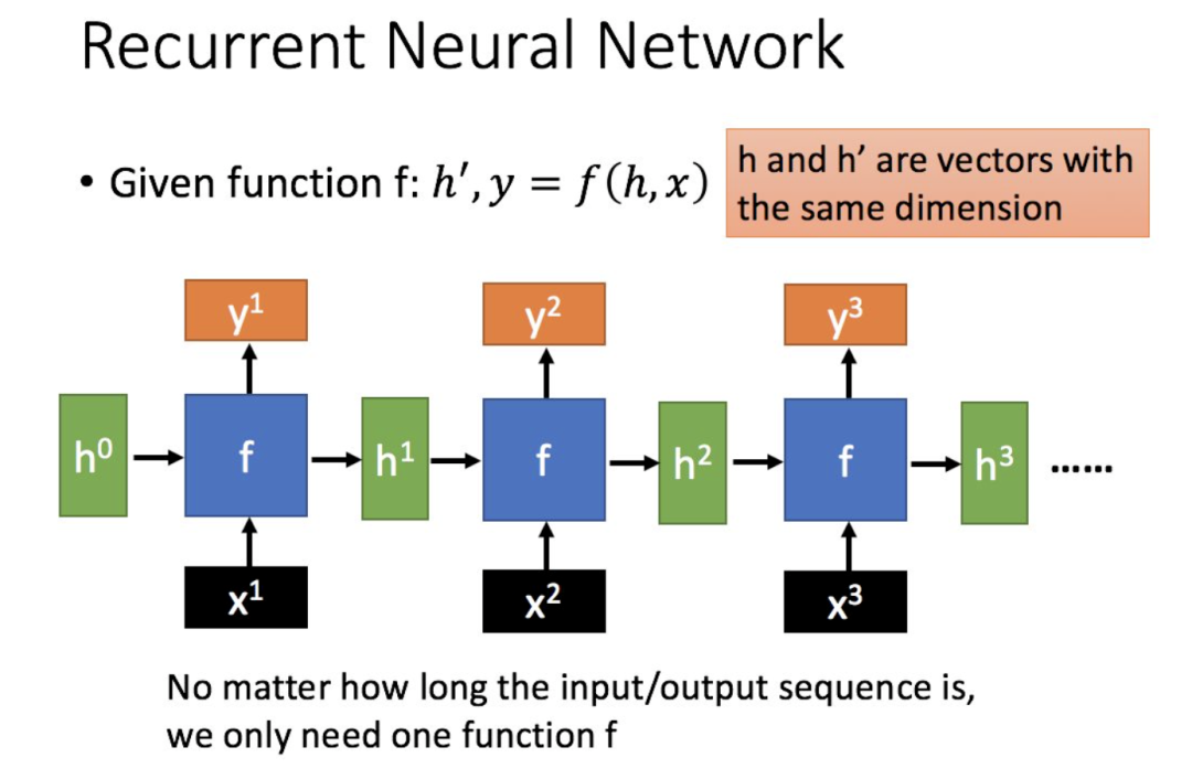
Recurrent Neural Network (RNN) is a type of neural network used for processing sequence data. Compared to regular neural networks, it can handle data that changes over sequences. For example, the meaning of a word can vary depending on the context mentioned earlier, and RNN can effectively address such issues.

1. Ordinary RNN

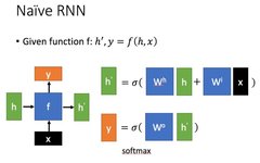
Let’s briefly introduce a typical RNN. Its main form is shown in the figure below (all images are from Professor Li Hongyi’s PPT):

Here:

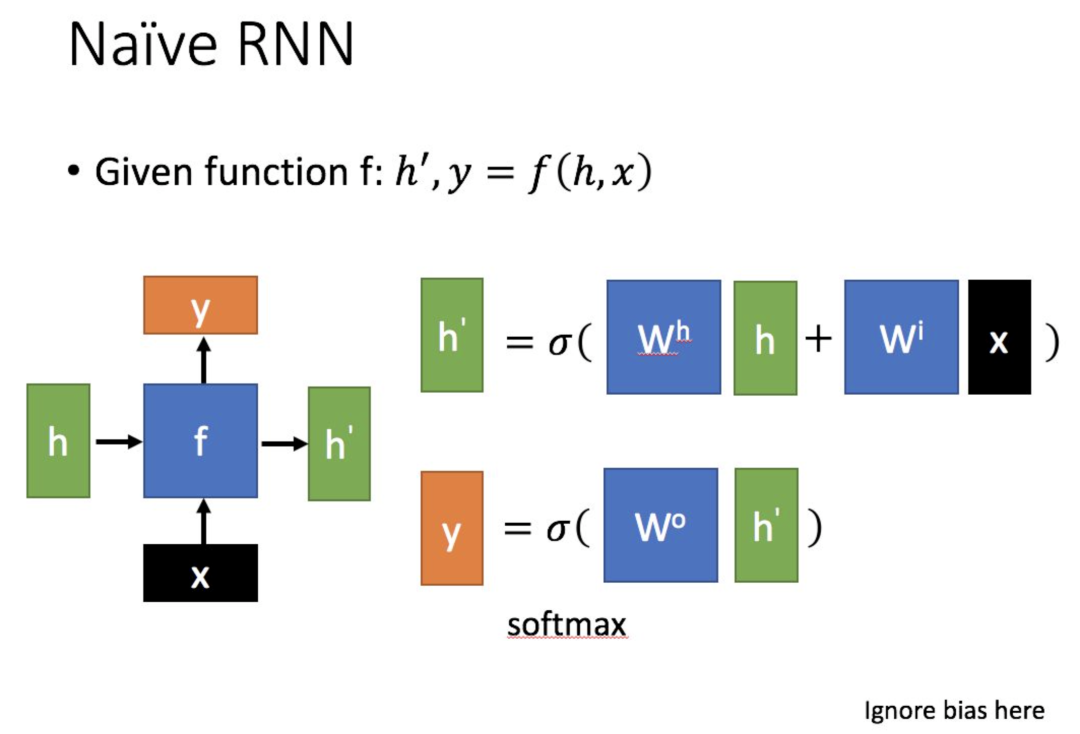
is the input data at the current state, represents the input received from the previous node.

is the output at the current node state, while is the output passed to the next node.

From the formula in the above figure, we can see that the output h’ is related to both x and h.

y is often calculated using h’ fed into a linear layer (primarily for dimensional mapping) and then classified using softmax to obtain the required data.

How y is calculated from h’ often depends on the specific model’s usage.

By inputting in sequence form, we can obtain the following form of RNN.

2. LSTM

2.1 What is LSTM

Long short-term memory (LSTM) is a special type of RNN designed to solve the problems of gradient vanishing and explosion during the training of long sequences. In simple terms, compared to ordinary RNNs, LSTM can perform better over longer sequences.

The structure of LSTM (right figure) differs from that of ordinary RNN mainly in its input and output as shown below.

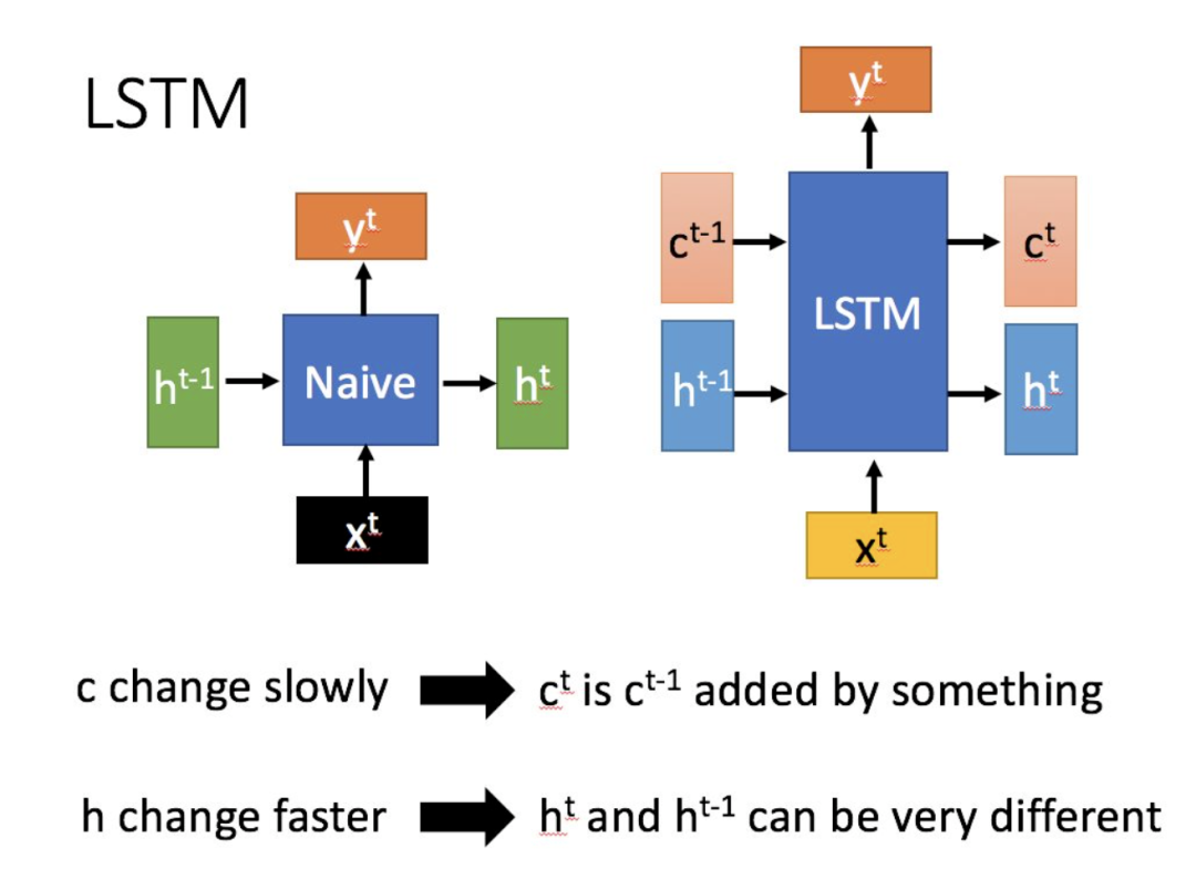
Compared to RNN, which has only one transmitted state , LSTM has two transmitted states, one (cell state) and one (hidden state). The in RNN is equivalent to the in LSTM.

For the transmitted state , it changes very slowly, with the output usually being the previous state plus some values.

Meanwhile, can often vary significantly across different nodes.

2.2 In-depth Look at LSTM Structure

Next, we will analyze the internal structure of LSTM in detail.

First, the current input and the previous state are concatenated to train and obtain four states.

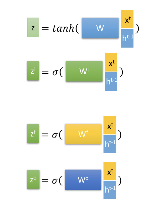
Here, , , are obtained by multiplying the concatenated vector by a weight matrix and then passing it through a sigmoid activation function to convert it into a value between 0 and 1, serving as a gating state. The is then transformed into a value between -1 and 1 using a tanh activation function (tanh is used here because it is treated as input data, not a gating signal).

Next, we will further introduce the use of these four states within LSTM (take note)

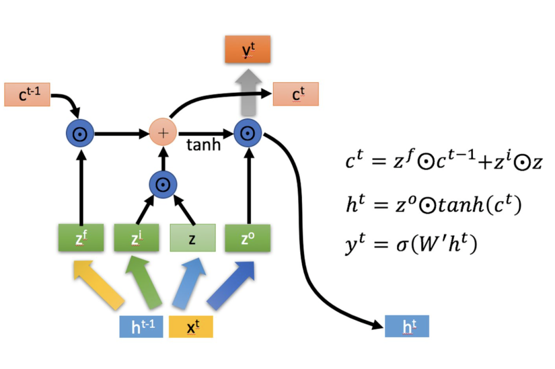
is Hadamard Product, which means multiplying corresponding elements in the matrices, hence the matrices must be of the same shape. denotes matrix addition.

There are mainly three phases in LSTM:

1. Forgetting Phase. This phase mainly performsselective forgetting of the input from the previous node. In simple terms, it “forgets the unimportant, remembers the important”.

Specifically, this is controlled by the forget gate computed as (f represents forget), which determines what from the previous state should be retained and what should be forgotten.

2. Selective Memory Phase. This phase selectively “remembers” the input. It focuses on recording the important aspects of the input while lessening the emphasis on the unimportant data. The current input is represented by the previously computed . The gating signal for selection is controlled by (i represents information).

Combining the results from the above two steps gives us the value to be passed to the next state, as shown in the first formula in the figure above.

3. Output Phase. This phase determines what will be considered the current output state. This is mainly controlled by . Additionally, the result from the previous phase is scaled (by a tanh activation function).

Similar to ordinary RNNs, the output is often ultimately derived from .

3. Summary

In summary, this is the internal structure of LSTM. It uses gating states to control the transfer of states, remembering what needs to be retained for a long time and forgetting unimportant information; unlike ordinary RNNs that can only “naively” stack memories in one way. This is particularly useful for many tasks requiring “long-term memory”.

However, due to the introduction of many components, the number of parameters increases, making training significantly more challenging. Therefore, we often use GRU, which achieves comparable results to LSTM but with fewer parameters, to build models for large training volumes.