In today's era, machines have successfully achieved 99% accuracy in understanding and recognizing features and objects in images. We see this every day - smartphones can recognize faces in the camera; the ability to search for specific photos using Google Image Search; scanning text from barcodes or books. All of this is made possible by Convolutional Neural Networks (CNNs), a specific type of neural network also known as convolutional networks.
If you are a deep learning enthusiast, you may have heard of Convolutional Neural Networks, and perhaps you have even developed some image classifiers yourself. Modern deep learning frameworks like TensorFlow and PyTorch make it easy to train machines to learn from images, but there are still some questions: How does data pass through the artificial layers of the neural network? How does the computer learn from it? One way to better explain Convolutional Neural Networks is by using PyTorch. So let’s dive deeper into CNNs by visualizing the images at each layer.


What are Convolutional Neural Networks?
Convolutional Neural Networks (CNNs) are a special type of neural network that performs particularly well on images. CNNs were proposed by Yan LeCun in 1998 and can recognize digits present in a given input image.
Before diving into using Convolutional Neural Networks, it is important to understand how neural networks work. Neural networks mimic how the human brain solves complex problems and finds patterns in a given dataset. Over the past few years, neural networks have swept through many machine learning and computer vision algorithms.
The basic model of a neural network consists of neurons organized in different layers. Each neural network has an input layer and an output layer, with many hidden layers added depending on the complexity of the problem. Once the data passes through these layers, the neurons learn and recognize patterns. This representation of the neural network is called a model. After training the model, we ask the network to make predictions based on the test data. If you are not familiar with neural networks, this article on deep learning with Python is a great starting point.
On the other hand, CNNs are a special type of neural network that performs particularly well on images. CNNs were proposed by Yan LeCun in 1998 and can recognize digits present in a given input image. Other applications of CNNs include speech recognition, image segmentation, and text processing. Before CNNs, Multi-Layer Perceptrons (MLPs) were used to build image classifiers.
Image classification refers to the task of extracting information categories from multi-band raster images. Multi-Layer Perceptrons require more time and space to search for information in images since each input feature needs to connect to every neuron in the next layer. CNNs replaced MLPs by using the concept of local connections, which involves connecting each neuron only to a local region of the input volume. By allowing different parts of the network to specialize in high-level features such as textures or repeated patterns, the number of parameters can be minimized. Confused? Don’t worry. Let’s compare how images are passed through a Multi-Layer Perceptron and a Convolutional Neural Network to better understand.
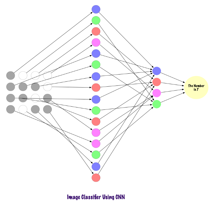
Consider the MNIST dataset, where the total number of inputs in the Multi-Layer Perceptron input layer will be 784 due to the size of the input images being 28×28 = 784. The network should be able to predict the digit present in the given input image, meaning the output could belong to any number in the range from 0 to 9 (1, 2, 3, 4, 5, 6, 7, 8, 9). In the output layer, we return the class scores; for example, if the given input is an image with the digit ‘3’, the corresponding neuron ‘3’ in the output layer will have a higher class score than other neurons. How many hidden layers do we need to include, and how many neurons should be in each layer? Here’s an example of coding an MLP:
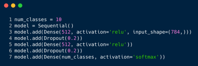
The code snippet above is implemented using a framework called Keras (temporarily ignoring syntax). It tells us that there are 512 neurons in the first hidden layer that connect to an input layer shaped like 784. After that hidden layer, there is a dropout layer that overcomes the issue of overfitting. The 0.2 indicates a 20% chance that a neuron will not be considered after the first hidden layer. Again, we add the same number of neurons (512) in the second hidden layer and then add another dropout. Finally, we end this set of layers with an output layer containing 10 classes. The class with the highest value will be the model’s prediction.
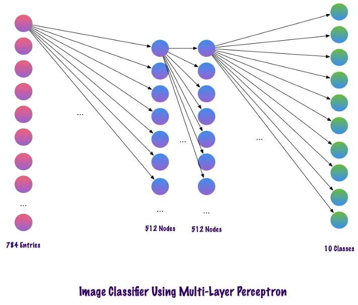
This is the multi-layer appearance of the network after defining all the layers. One downside of this Multi-Layer Perceptron is that the fully connected layers require more time and space for the network to learn. MLPs only accept vectors as input.
Convolutional layers do not use fully connected layers but instead use sparse connection layers, meaning they accept matrices as input, which is more advantageous than MLPs. Input features connect to local coding nodes. In MLPs, each node is responsible for gaining an understanding of the entire image. In CNNs, we break the image down into regions (local areas of pixels). Each hidden node must report to the output layer, where the output layer combines the received data to find patterns. The following diagram shows how local connections are made across layers.
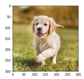
Before we understand how CNNs find information in images, we need to understand how features are extracted. Convolutional Neural Networks use different layers, each storing features from the images. For example, consider a picture of a dog. Whenever the network needs to classify the dog, it should recognize all the features – eyes, ears, tongue, legs, etc. These features are decomposed and identified in the local layers of the network using filters and kernels.
Unlike humans who understand images through their eyes, computers use a set of pixel values ranging from 0 to 255 to understand pictures. The computer looks at these pixel values and understands them. At first glance, it doesn’t know objects or colors; it only recognizes pixel values, which is all images are to computers.
After analyzing the pixel values, the computer slowly begins to understand whether the image is grayscale or color. It knows the difference because a grayscale image has only one channel, where each pixel represents the intensity of one color. Zero represents black, and 255 represents white, with other variations of black and white, i.e., the shades of gray in between. On the other hand, a color image has three channels – red, green, and blue. They represent the intensity of three colors (3D matrix), and when the values change simultaneously, it creates a wide range of colors! After determining the color attributes, the computer identifies the curves and contours of objects in the image.
This process can be explored using PyTorch in Convolutional Neural Networks to load datasets and apply filters to images. Here’s a code snippet. (This code can be found on GitHub)
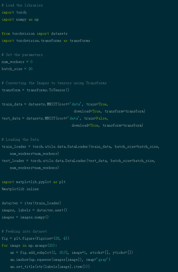
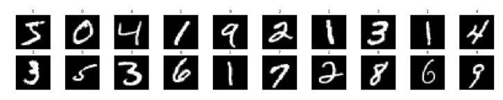
Now, let’s see how to input a single image into the neural network.
(This code can be found on GitHub)
img = np.squeeze(images[7])
fig = plt.figure(figsize = (12,12))
ax = fig.add_subplot(111)
ax.imshow(img, cmap='gray')
width, height = img.shape
thresh = img.max()/2.5
for x in range(width):
    for y in range(height):
        val = round(img[x][y],2) if img[x][y] !=0 else 0
        ax.annotate(str(val), xy=(y,x),
            color='white' if img[x][y]<thresh else 'black')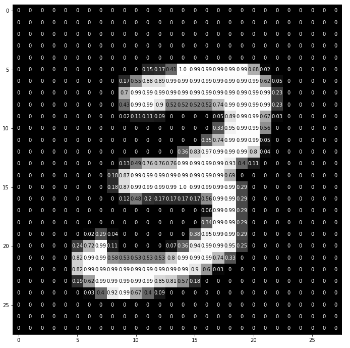
This is how the digit ‘3’ is broken down into pixels. From a set of handwritten digits, we randomly select ‘3’, showing pixel values. Here, ToTensor() normalizes the actual pixel values (0–255) and restricts them to 0 to 1. Why? Because this makes calculations in later parts easier, whether in interpreting the image or finding common patterns present in the image.
In Convolutional Neural Networks, pixel information in images is filtered. Why do we need filters at all? Just like children, computers need to go through a learning process to understand images. Fortunately, this doesn’t take years! Computers accomplish this task by learning from scratch and then gradually moving to the whole. Therefore, the network must first know all the raw parts of the image, such as edges, contours, and other low-level features. Once these are detected, the computer can handle more complex functions. In short, low-level features must be extracted first, then mid-level features, and finally high-level features. Filters provide a way to extract information.
Specific filters can be used to extract low-level features, which are also a set of pixel values similar to the image. They can be understood as the weights connecting the layers in the CNN. By multiplying these weights or filters with the input, an intermediate image is obtained, representing the computer’s partial understanding of the image. These by-products are then multiplied with more filters to expand the view. This process and the detection of features continue until the computer understands what it looks like.
You can use many filters according to your needs. You might need to blur, sharpen, deepen, perform edge detection, etc. – all are filters.
Let’s look at some code snippets to understand the functionality of filters.

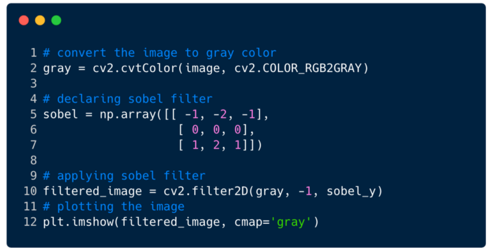
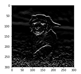
This is how the image looks after applying the filter. In this case, we used the Sobel filter.
Complete Convolutional Neural Networks (CNNs)
We have learned how filters extract features from images, but to complete the entire Convolutional Neural Network, we need to understand the layers used to design CNNs. The layers in a Convolutional Neural Network are called:
1. Convolutional Layer
2. Pooling Layer
3. Fully Connected Layer
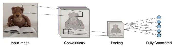
Using these 3 layers, a classifier like this can be constructed:
Function of Each Layer in CNN
Now let’s take a look at what each layer is used for
Convolutional Layer — The Convolutional Layer (CONV) performs convolution operations using filters while scanning the dimensions of the input image. Its hyperparameters include filter size, usually set to 2×2, 3×3, 4×4, 5×5 (but not limited to these sizes), and stride (S). The output result (O) is called the feature map or activation map, which contains all the features computed from the input layer and the filters. The following diagram describes the feature map produced when applying convolution:
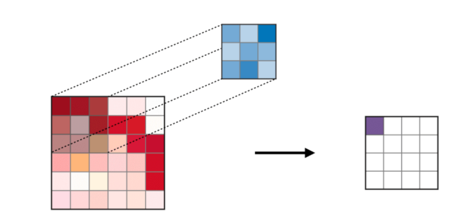
Convolution Operation
Pooling Layer — The Pooling Layer (POOL) is used for down-sampling features and is typically applied after the Convolutional Layer. The two common pooling operations are max pooling and average pooling, which take the maximum and average values of the features, respectively. The following diagram describes the basic principles of pooling:
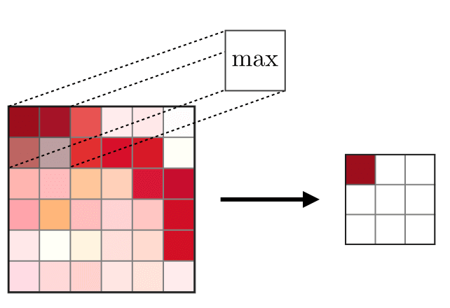
Max Pooling
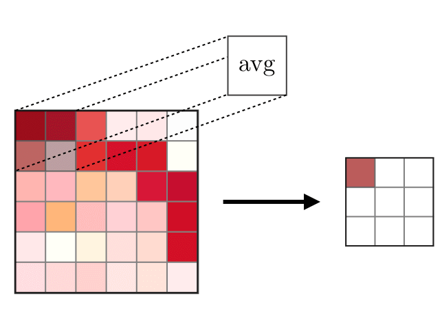
Average Pooling
Fully Connected Layer — The Fully Connected Layer (FC) acts on a flattened input, where each input is connected to all neurons. Fully Connected Layers are typically used at the end of the network to connect hidden layers to the output layer, which helps optimize class scores.
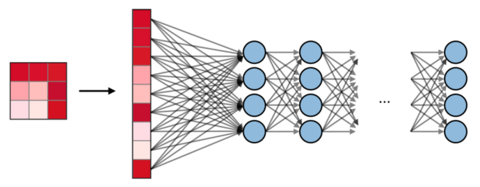
Fully Connected Layer
We have a better understanding of the functions of CNNs, and now let’s implement it using Facebook’s PyTorch framework.
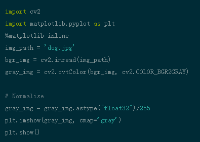
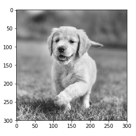
Step 1: Load the input image. We will use Numpy and OpenCV. (This code can be found on GitHub)
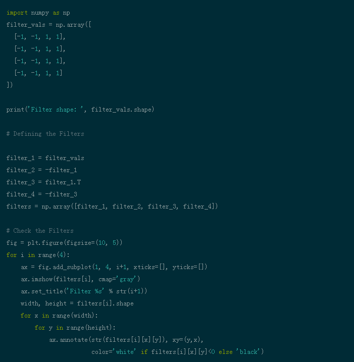
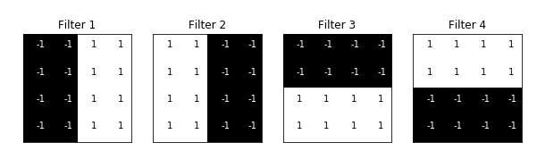
Step 2: Visualize the filters to better understand the filters we will use. (This code can be found on GitHub)
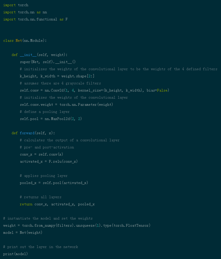
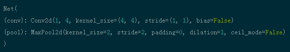
Step 3: Define the Convolutional Neural Network. This CNN has convolutional layers and max pooling layers, and weights are initialized using the filters mentioned above: (This code can be found on GitHub)
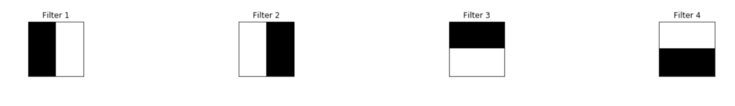
Step 4: Visualize the filters. Take a quick look at the filters being used. (This code can be found on GitHub)
def viz_layer(layer, n_filters= 4):    fig = plt.figure(figsize=(20, 20))
    for i in range(n_filters):        ax = fig.add_subplot(1, n_filters, i+1)        ax.imshow(np.squeeze(layer[0,i].data.numpy()), cmap='gray')        ax.set_title('Output %s' % str(i+1))
fig = plt.figure(figsize=(12, 6))
fig.subplots_adjust(left=0, right=1.5, bottom=0.8, top=1, hspace=0.05, wspace=0.05)
for i in range(4):    ax = fig.add_subplot(1, 4, i+1, xticks=[], yticks=[])    ax.imshow(filters[i], cmap='gray')    ax.set_title('Filter %s' % str(i+1))
gray_img_tensor = torch.from_numpy(gray_img).unsqueeze(0).unsqueeze(1)
Filters:
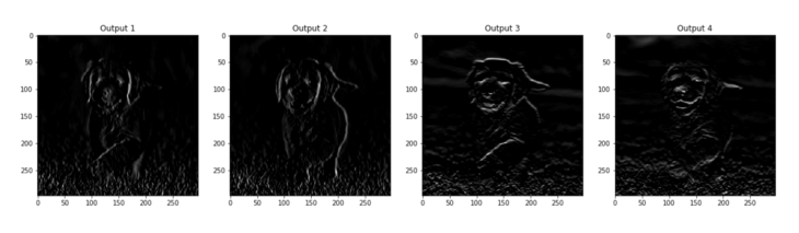
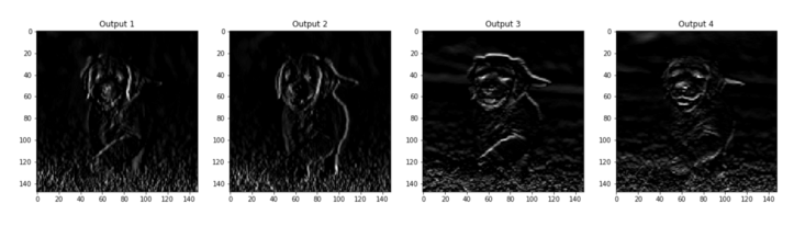
Step 5: Cross-layer filter outputs. The images output in the CONV and POOL layers are shown below.
viz_layer(activated_layer)
viz_layer(pooled_layer)