Are you a new friend? Remember to click the blue text to follow me~
Introduction
This article mainly discusses convolution operations and their derived operations, which I would call the strongest! Since its introduction, convolution has gradually become an essential part of modern CNN networks due to its excellent feature extraction capability, triggering a wave of research on methods based on deep learning in computer vision!

1. Classic Convolution
Before explaining how convolution works, we need to understand why we use convolution and what the advantages of convolutional neural networks are compared to fully connected neural networks.
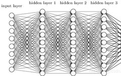
1.1 Defects of Fully Connected Neural Networks
Before the advent of convolutional neural networks, deep learning used fully connected neural networks. What is full connection? Full connection means that all neurons in adjacent layers are connected, which undoubtedly leads to a huge number of parameters. This is one of the problems with fully connected neural networks. However, this is not fatal; the most fatal problem is that fully connected neural networks “ignore” the shape of the data. What does this mean? Let’s look at the following case.
For example, when the input data is an image, the image usually has a 3D shape in height, width, and channel direction. However, when inputting to a fully connected layer, the 3D data needs to be flattened into 1D data. In fact, in the case of the MNIST dataset, the input image has a shape of (1, 28, 28) with 1 channel, height of 28 pixels, and width of 28 pixels, but it is arranged in a single column and input to the fully connected neural network as 784 data points.
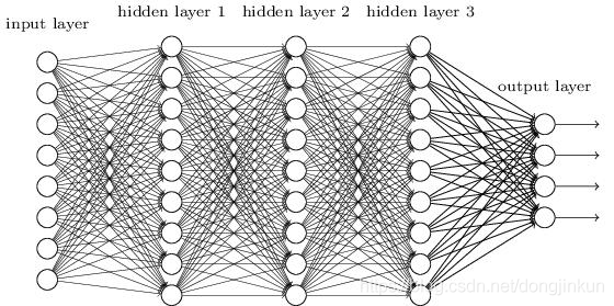
Assuming the input image has a 3D shape, this shape should contain important spatial information; otherwise, there would be no need for it to be 3D. This information may include that neighboring pixels in space have similar values, that there are close correlations between the RGB channels, and that there is little correlation between pixels that are far apart. There may be essential patterns hidden in the 3D shape that are worth extracting. However, because fully connected layers ignore the shape, treating all input data as the same neuron (neurons in the same dimension), they cannot utilize shape-related information. This is the most fatal problem of fully connected neural networks.
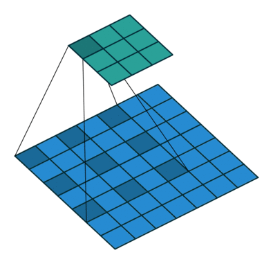
1.2 How Convolution Works
step1: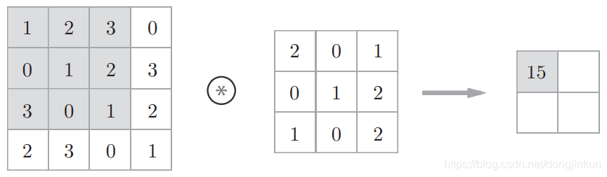 step2:
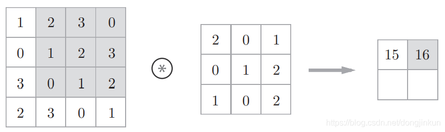 step3:
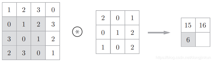 step4:
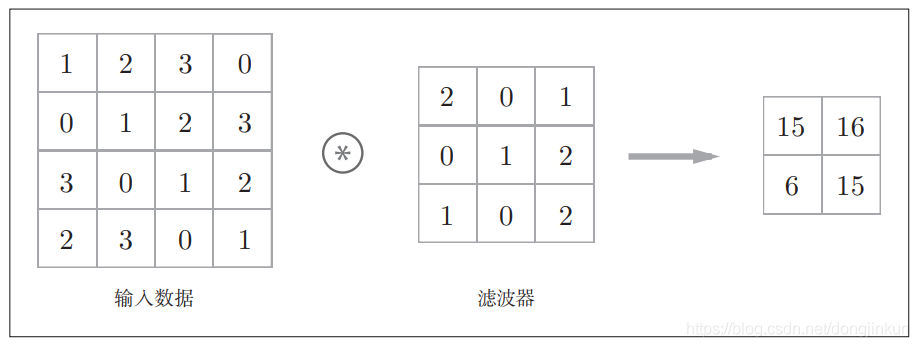
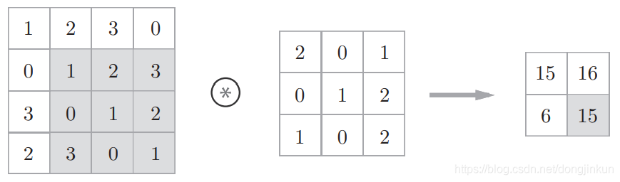 Through the following two images, we can understand the working principle of convolution more intuitively.

1.3 How to Calculate Output Size
Assuming the input size is (H, W), filter size is (FH, FW), output size is (OH, OW), padding is P, and stride is S, the output size can be calculated using the following formula.
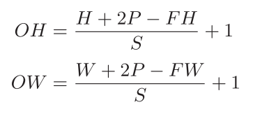
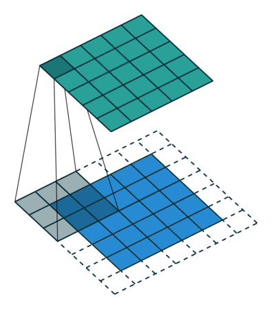
1.4 How to Convolve 3D Data
When conducting experiments, the input is usually an RGB image with 3 channels, which is the most common scenario, so we need to explain how 3D data is convolved. Let’s look at the following case, which is very simple but absolutely classic: step1:
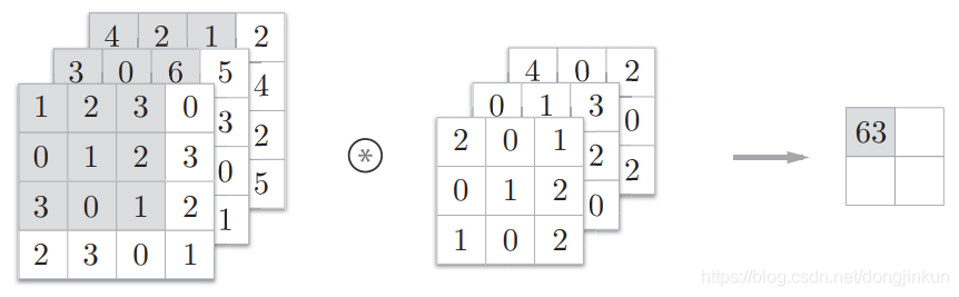 step2:
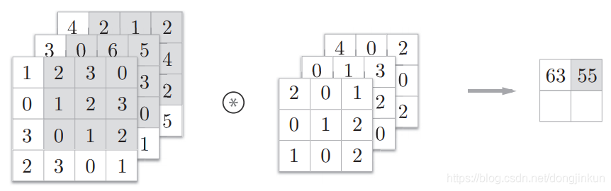 step3:
 step4:
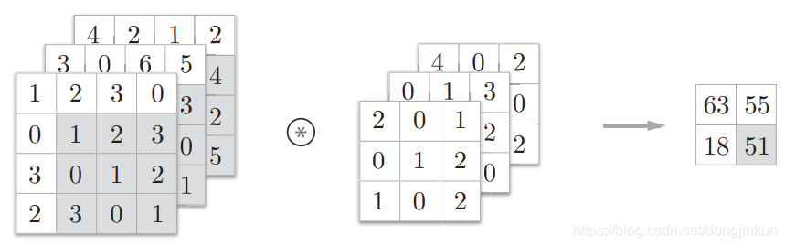 Note: It is important to note that
In the convolution operation of 3D data, the number of channels in the input data and the filter must be the same. In the above example, both the input data and the filter have 3 channels. The filter size can be set to any value, but the filter size for each channel must be the same.
1.5 Recommended Papers
★
“Gradient-Based Learning Applied to Document Recognition”
”
★
“ImageNet Classification with Deep Convolutional Neural Networks”
”
2. Dilated Convolution
2.1 Operating Principle of Dilated Convolution
Dilated convolution, also known as dilated convolution, is a very important concept in convolutional neural networks. The purpose of dilated convolution is to expand the receptive field to improve model performance. The operating principle of dilated convolution is very similar to convolution, with the only difference being that dilated convolution introduces the concept of dilated rate. One can consider ordinary convolution as a special case of dilated convolution, where the dilated rate of ordinary convolution is set to 1.
 The following are examples of dilated convolution with dilated rates of 1, 6, and 24:
2.2 Recommended Papers
For a detailed introduction to dilated convolution, you can refer to the famous DeepLab series of papers, including DeepLab v2 and DeepLab v3.
★
“DeepLab: Semantic Image Segmentation with Deep Convolutional Nets, Atrous Convolution, and Fully Connected CRFs”
”
★
“Rethinking Atrous Convolution for Semantic Image Segmentation”
”
3. Transposed Convolution
Transposed convolution, also known as deconvolution, is, as the name suggests, the operation of transposed convolution is the opposite of convolution. Transposed convolution is commonly used in the upsampling phase. What is upsampling? There will be a dedicated article to introduce common upsampling methods, including transposed convolution, nearest neighbor interpolation, bilinear interpolation, etc. Since transposed convolution is more focused on the upsampling phase, this article will be more focused on convolution methods for feature extraction, so transposed convolution will be detailed in the subsequent upsampling article.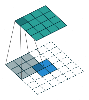
4. Separable Convolution
Separable convolution is divided into spatial separable convolution and depthwise separable convolution.
4.1 Spatial Separable Convolution
Spatial separable convolution is designed using the properties of matrix multiplication. Please see the following case. Assuming the convolution kernel size is 33, this convolution kernel can be viewed as a multiplication of a 31 vector and a 1*3 vector. The benefit of this is to reduce the model parameters and decrease the amount of multiplication computation.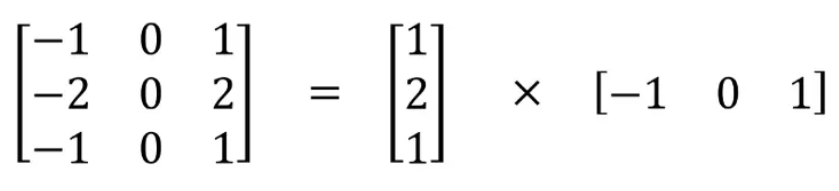
4.2 Depthwise Separable Convolution
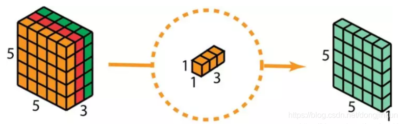
Depthwise separable convolution is one of the most remarkable operations in convolutional neural networks, which I would gladly call it. Depthwise separable convolution consists of two steps, the first step is to use each convolution kernel to convolve with one channel of the input image respectively, and the second step is to expand the depth, as shown in the diagram (image source).
Ordinary convolution uses a convolution kernel with the same number of channels as the input image to output a feature map with 1 channel, while depthwise separable convolution uses 3 convolution kernels (each convolution kernel size is 3 x 3 x 1) instead of a convolution kernel of size 3 x 3 x 3. Each convolution kernel only convolves with one channel of the input image, resulting in a mapping of size 5 x 5 x 1 each time. Then these mappings are stacked together to create a 5 x 5 x 3 image, ultimately resulting in an output image of size 5 x 5 x 3. In this way, the depth of the image remains the same as before.
The second step of depthwise separable convolution is to expand the depth, where we use a convolution kernel of size 1x1x3 for a 1×1 convolution. Each 1x1x3 convolution kernel convolves with a 5 x 5 x 3 input image to produce a mapping of size 5 x 5 x 1.
 After performing 128 times of 1×1 convolution, we can obtain a feature map of size 5 x 5 x 128.
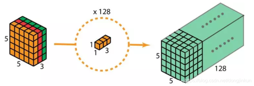 The complete process of depthwise separable convolution is shown in the following diagram.
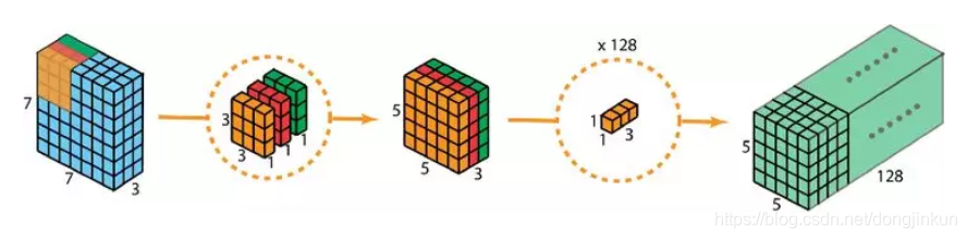
4.3 Recommended Papers
★
“Xception: Deep Learning with Depthwise Separable Convolutions”
”
5. 3D Convolution
From the name, we can understand the general meaning of 3D convolution. Ordinary convolution performs convolution operations in 2D space, while 3D convolution simply performs convolution operations in 3D space. As can be seen, 3D convolution is merely an extension of 2D convolution in the channel dimension. The 3D convolution kernel can move along 3 directions (height, width, and the image’s channel), which is not significantly different from 2D convolution, as shown in the following image (image source):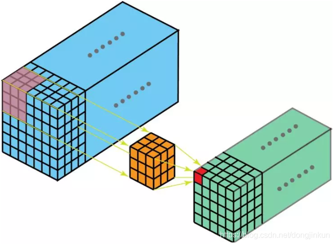
6. Group Convolution
6.1 Principle of Group Convolution
Group convolution was first proposed in the famous AlexNet. For a detailed understanding of AlexNet, you can refer to my blog on AlexNet, which is very detailed. The introduction of group convolution was to solve the problem of insufficient GPU computing power. When training AlexNet, convolution operations could not all be processed on the same GPU, so the author divided the feature maps among multiple GPUs for processing, and finally merged the results from multiple GPUs. In ordinary convolution, all convolution kernels convolve the input at once.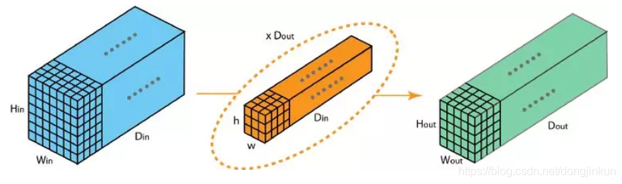 In group convolution, the convolution kernels are split into different groups, each responsible for performing ordinary convolution operations with a certain depth. The following image can more intuitively illustrate the operating principle of group convolution.
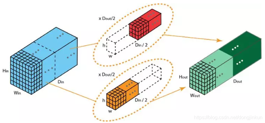
6.2 Recommended Papers
I recommend reading the following paper AlexNet, which can be regarded as one of the pioneers of convolutional neural networks, very classic.
★
“ImageNet Classification with Deep Convolutional Neural Networks”
”
References
★
“Introduction to Deep Learning – Theory and Implementation Based on Python”
“ImageNet Classification with Deep Convolutional Neural Networks”
“Gradient-Based Learning Applied to Document Recognition”
“ImageNet Classification with Deep Convolutional Neural Networks”
https://blog.csdn.net/gwplovekimi/article/details/89890510
“Xception: Deep Learning with Depthwise Separable Convolutions”