Click the above “Beginner Learning Visuals“, select Star or Pin“
Heavyweight resources delivered instantly
Facial expressions are an important way of communication among humans.
In artificial intelligence research, deep learning techniques have become a powerful tool to enhance human-computer interaction. The analysis and assessment of facial expressions and emotions in psychology involves evaluating the predictions of individual or group emotions.
This study aims to develop a system that can predict and classify facial emotions using Convolutional Neural Network (CNN) algorithms and feature extraction techniques.
The process includes three main stages: data preprocessing, facial feature extraction, and facial emotion classification. By adopting the Convolutional Neural Network (CNN) algorithm, the system accurately predicts facial expressions with a success rate of 62.66%.
The performance of the algorithm is evaluated using the FER2013 database, which is a publicly available dataset containing 35,887 grayscale facial images of size 48×48, each representing a different emotion.
Now let’s start with the coding.
!pip install scikit-plot
This code uses pip to install the scikit-plot package, which is a Python package that provides a range of useful tools for visualizing the performance of machine learning models.
Specifically, scikit-plot provides various functions to generate common plots used in model evaluation, such as ROC curves, precision-recall curves, confusion matrices, etc.
After executing the command “!pip install scikit-plot” in a Python environment, you should be able to import and use scikit-plot functions in your code.
import pandas as pd
import numpy as np
import scikitplot
import random
import seaborn as sns
import keras
import os

from matplotlib import pyplot
import matplotlib.pyplot as plt

import tensorflow as tf
from tensorflow.keras.utils import to_categorical
import warnings
from tensorflow.keras.models import Sequential

from keras.callbacks import EarlyStopping
from keras import regularizers
from keras.callbacks import ModelCheckpoint,EarlyStopping

from tensorflow.keras.optimizers import Adam,RMSprop,SGD,Adamax

from keras.preprocessing.image import ImageDataGenerator,load_img
from keras.utils.vis_utils import plot_model
from keras.layers import Conv2D, MaxPool2D, Flatten,Dense,Dropout,BatchNormalization,MaxPooling2D,Activation,Input

from sklearn.model_selection import train_test_split
from sklearn.preprocessing import StandardScaler
warnings.simplefilter("ignore")

from keras.models import Model

from sklearn.model_selection import train_test_split
from sklearn.metrics import accuracy_score

from keras.regularizers import l1, l2
import plotly.express as px
from matplotlib import pyplot as plt

from sklearn.metrics import confusion_matrix
from sklearn.metrics import classification_report
This code imports various Python libraries and modules commonly used in machine learning and deep learning tasks.
These libraries include pandas, numpy, scikit-plot, random, seaborn, keras, os, matplotlib, tensorflow, and scikit-learn.
Each import statement imports a set of specific tools or functions needed to perform machine learning or deep learning tasks, such as data manipulation, data visualization, model building, and performance evaluation.
Overall, this code prepares the necessary tools and modules needed to perform various machine learning and deep learning tasks (such as data preprocessing, model training, and model evaluation).
Download the code from here: http://onepagecode.s3-website-us-east-1.amazonaws.com/
Load Dataset
data = pd.read_csv("../input/fer2013/fer2013.csv")
data.shape
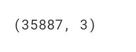
This code uses pandas’ read_csv() function to read a CSV file named “fer2013.csv” located in the “../input/fer2013/” directory and assigns the resulting DataFrame to a variable named data.
Then, it calls the shape attribute on the DataFrame to retrieve its dimensions, which will return a tuple of the form. This line of code will output the number of rows and columns in the DataFrame data as (rows, columns).
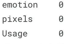
data.isnull().sum()
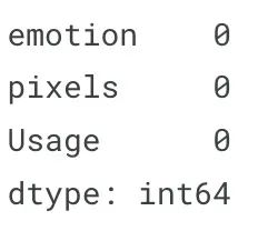
This code will return the total number of missing values in each column of the DataFrame data.
The isnull() method of the DataFrame returns a boolean DataFrame indicating whether each element in the original DataFrame is missing. The sum() method is then applied to this boolean DataFrame, which returns the total number of missing values in each column.
This is a quick way to check if there are any missing values in the DataFrame. If there are missing values, you may need to impute or delete them before using the data for modeling.
data.head()
This code will return the first 5 rows of the DataFrame data.
The head() method of the DataFrame returns the first n rows of the DataFrame (default is n=5). This is a useful way to quickly browse the data in the DataFrame, especially when working with large datasets.
The output will display the first 5 rows of the DataFrame data, which may include column names and the first few rows of data, depending on the structure of the DataFrame.
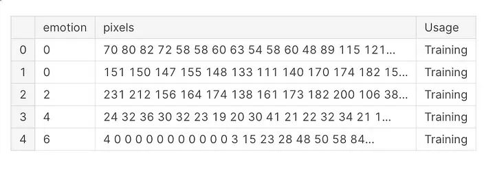
Output of data head
Data Preprocessing
CLASS_LABELS  = ['Anger', 'Disgust', 'Fear', 'Happy', 'Neutral', 'Sadness', "Surprise"]
fig = px.bar(x = CLASS_LABELS,
             y = [list(data['emotion']).count(i) for i in np.unique(data['emotion'])] ,
             color = np.unique(data['emotion']) ,
             color_continuous_scale="Emrld")
fig.update_xaxes(title="Emotions")
fig.update_yaxes(title = "Number of Images")
fig.update_layout(showlegend = True,
    title = {
        'text': 'Train Data Distribution ',
        'y':0.95,
        'x':0.5,
        'xanchor': 'center',
        'yanchor': 'top'})
fig.show()
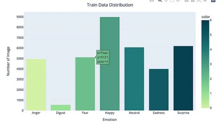
This code uses the Plotly Express library to create a bar chart that shows the distribution of emotions in the DataFrame data.
First, a list of class labels is defined in CLASS_LABELS, corresponding to different emotions in the dataset.
Then, the px.bar() function is called, where the x-axis represents the class labels and the y-axis represents the number of images for each emotion. The color parameter is set to different emotional classes, and the color_continuous_scale parameter is set to “Emrld”, which is a predefined color scale in Plotly Express.
Next, various update_ methods are called to modify the layout and appearance of the plot. For example, update_xaxes() and update_yaxes() are used to set the titles for the x-axis and y-axis, respectively. update_layout() is used to set the title of the plot and its position.
Finally, the show() method is called on the figure object to display the plot.
The output will show a bar chart that displays the number of images for each emotion in the DataFrame data, with each emotion color-coded according to the specified color scale.
Random Shuffle Data
data = data.sample(frac=1)
The sample() method of the DataFrame is used to randomly sample a small portion of the rows in the DataFrame and specifies frac to return the portion of rows (in this case, frac=1, which means all rows will be returned). When frac=1, the sample() method effectively shuffles the rows in the DataFrame.
This is a common operation in machine learning and deep learning tasks, and it is important to randomly shuffle the data to prevent any biases that might be introduced when the data has any inherent order or structure.
One Hot Encoding
labels = to_categorical(data[['emotion']], num_classes=7)
The output is a numpy array with the shape (n_samples, n_classes), where:
-
n_samplesis the number of samples in the DataFrame -
n_classesis the number of unique classes in the data (in this case, 7) -
Each row of the array datarepresents the One Hot encoded labels for a single sample in the DataFrame.
train_pixels = data["pixels"].astype(str).str.split(" ").tolist()
train_pixels = np.uint8(train_pixels)
This code preprocesses the pixel values in the pixels column of the DataFrame.
First, the astype() method is used to convert the pixels column to string data type, which allows the split() method to be called on each row of the column.
Next, the split() method is called on each row of the pixels column to split the pixel values into a list of strings. The resulting list is then converted to a numpy array using tolist().
Finally, the np.uint8() is called on the numpy array to convert the pixel values from strings to unsigned 8-bit integers, which is the data type typically used to represent image pixel values.
The output is a numpy array with the shape (n_samples, n_pixels), where n_samples is the number of samples in the DataFrame, and n_pixels is the number of pixels in each image in the data. Each row of the array data represents the pixel values for a single image in the DataFrame.
Normalization
pixels = train_pixels.reshape((35887*2304,1))
This code reshapes the train_pixels numpy array from a 3D shape array (n_samples, n_rows, n_columns) to a 2D shape array (n_samples*n_row, 1).
The reshape() method of the numpy array is used to change its shape. In this case, the train_pixels array is flattened by reshaping it into a 2D array with one column.
The resulting pixel array has the shape of (n_samples*n_rows, 1), where n_samples is the number of samples in the DataFrame, n_rows is the number of rows in each image, and 1 represents the flattened pixel values for each image in the DataFrame. Each row of the array represents a single pixel value for a single image in the DataFrame.
scaler = StandardScaler()
pixels = scaler.fit_transform(pixels)
This code applies normalization to the pixel numpy array using the StandardScaler() function from scikit-learn.
The StandardScaler() function is a preprocessing step that scales each feature of the data (in this case, each pixel value) to have a mean of 0 and a variance of 1. This is a common technique in machine learning and deep learning tasks to ensure that each feature contributes equally to the model.
Then, the fit_transform() method of the StandardScaler() object is called on the pixel numpy array, which computes the mean and standard deviation of the data and scales the data accordingly. The resulting scaled data is then assigned back to the pixel numpy array.
The output is a numpy array with the same shape as the original pixels array, but each pixel value has been normalized.
Reshape Data (48, 48)
pixels = train_pixels.reshape((35887, 48, 48,1))
This code reshapes the train_pixels numpy array from a 2D shape array (n_samples*n_rows, 1) to a 4D shape array (n_samples, n_rows, n_columns, n_channels).
The reshape() method of the numpy array is used to change its shape. In this case, the train_pixels array is reshaped into a 4D array with one channel.
The resulting pixel array has the shape of (n_samples, n_rows, n_columns, n_channels), where n_samples is the number of samples in the DataFrame, n_row is the number of rows in each image, n_column is the number of columns in each image, and n_channel represents the number of color channels in each image.
Since the original dataset is grayscale, n_channels is set to 1. Each element of the pixel array represents the pixel values for a single grayscale image in the DataFrame.
Train-Test-Validation Split
Now, we have 35,887 images, each containing 48×48 pixels. We will split the data into training, testing, and validation sets, providing 10% for evaluation and validation.
X_train, X_test, y_train, y_test = train_test_split(pixels, labels, test_size=0.1, shuffle=False)
X_train, X_val, y_train, y_val = train_test_split(X_train, y_train, test_size=0.1, shuffle=False)
This code uses the train_test_split() function from scikit-learn to split the preprocessed image data pixels and one-hot encoded labels into training, validation, and testing sets.
The train_test_split() function randomly splits the data into training and testing subsets based on the test_size parameter, which specifies the portion of data to apply for testing. In this case, test_size=0.1, meaning 10% of the data will be used for testing.
The shuffle parameter is set to False to preserve the original order of samples in the DataFrame.
The resulting X_train, X_val, and X_test arrays contain the pixel values for the training set, validation set, and testing set, respectively. The y_train, y_val, and y_test arrays contain the corresponding one-hot encoded labels for each set.
Again, train_test_split() is used to further split the training set into training and validation sets with test_size=0.1. This divides the data into 80% for training, 10% for validation, and 10% for testing.
print(X_train.shape)
print(X_test.shape)
print(X_val.shape)
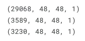
After splitting the data into training, validation, and testing sets, these lines of code print the shapes of the X_train, X_test, and X_val arrays.
The shape attribute of the numpy array returns a tuple of the dimensions of the array. In this case, the shapes of X_train, X_test, and X_val arrays will depend on the number of samples in each set and the dimensions of each sample.
The output will display the shapes of the arrays in the format (n_samples, n_rows, n_columns, n_channel), where n_samples is the number of samples in the set, n_rows is the number of rows in each image, n_columns is the number of columns in each image, and n_channel represents the number of color channels in each image.
With the help of this plotting code, we can see some samples from the training data containing one sample from each class.
plt.figure(figsize=(15,23))
label_dict = {0 : 'Angry', 1 : 'Disgust', 2 : 'Fear', 3 : 'Happiness', 4 : 'Sad', 5 : 'Surprise', 6 : 'Neutral'}
i = 1
for i in range (7):
    img = np.squeeze(X_train[i])
    plt.subplot(1,7,i+1)
    plt.imshow(img)
    index = np.argmax(y_train[i])
    plt.title(label_dict[index])
    plt.axis('off')
    i += 1
plt.show()
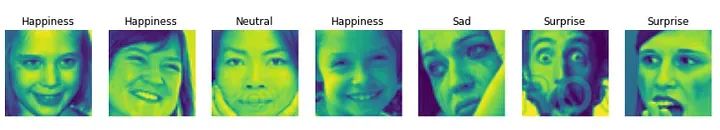
This code creates a 7×1 grid of subplots of images from the training set using the plt.subplots() function from matplotlib.
The squeeze() method of the numpy array is used to remove any single-dimensional entries from the shape of the array, effectively converting a 4D array into a 3D array.
For each subplot, the imshow() function is used to display the corresponding image, and the title() function is used to display the corresponding label.
The axis() function is used to turn off the axes for each subplot.
The output is a visualization of the first 7 images in the training set, along with their corresponding labels.
Data Augmentation Using Image Data Generator
We can perform data augmentation to obtain more data for training and validating our model to prevent overfitting. Data augmentation can be done on both the training and validation sets as it helps the model to become more general and robust.
datagen = ImageDataGenerator(  width_shift_range = 0.1,
                               height_shift_range = 0.1,
                               horizontal_flip = True,
                               zoom_range = 0.2)
valgen = ImageDataGenerator(   width_shift_range = 0.1,
                               height_shift_range = 0.1,
                               horizontal_flip = True,
                               zoom_range = 0.2)
This code creates two ImageDataGenerator objects, datagen and valgen, which will be used for data augmentation during training and validation.
The ImageDataGenerator class is a Keras preprocessing utility that can perform various types of image augmentation in real-time, such as shifting, flipping, rotating, and zooming.
The datagen object includes several augmentation techniques:
-
width_shift_rangeandheight_shift_rangeshift the image randomly by a maximum of 10% of the image width and height, respectively. -
horizontal_fliprandomly flips the image horizontally. -
zoom_rangerandomly zooms the image by up to 20%.
The valgen object contains the same augmentation techniques as datagen but is applied only to the validation set during training.
By applying data augmentation during training, the model will be exposed to a larger and more diverse training dataset, which helps prevent overfitting and improves the model’s ability to generalize to new data.
datagen.fit(X_train)
valgen.fit(X_val)
These lines of code fit the ImageDataGenerator objects datagen and valgen to the training and validation data, respectively.
The fit() method of the ImageDataGenerator object calculates any internal statistics needed to perform data augmentation, such as the mean and variance of the pixel values. In this case, the fit() method is called on datagen and valgen with the training and validation sets as inputs to compute these statistics.
Once the ImageDataGenerator objects are fitted to the data, they can be used to apply data augmentation in real-time during training and validation.
train_generator = datagen.flow(X_train, y_train, batch_size=64)
val_generator = datagen.flow(X_val, y_val, batch_size=64)
These lines of code create two ImageDataGenerator iterators, train_generator and val_generator, which will be used to generate a batch of augmented data during training and validation.
The flow() method of the ImageDataGenerator object takes numpy arrays of input data and labels and dynamically generates a batch of augmented data.
In this case, the flow() method on datagen creates the train_generator, with the training data X_train and y_train, with a batch size of 64. The val_generator is created using the same method on valgen, with the validation data X_val and y_val, also with a batch size of 64.
During training, the train_generator (iterator) will be used to dynamically generate a batch of augmented data for each training epoch. Similarly, the val_generator iterator will be used to generate a batch of augmented data for each validation epoch.
Code Download
http://onepagecode.s3-website-us-east-1.amazonaws.com/
Design Model
Convolutional Neural Network (CNN) Model
The CNN model consists of many layers with different units, such as convolutional layers, max pooling layers, batch normalization, and dropout layers to regularize the model.
def cnn_model():
  model= tf.keras.models.Sequential()
  model.add(Conv2D(32, kernel_size=(3, 3), padding='same', activation='relu', input_shape=(48, 48,1)))
  model.add(Conv2D(64,(3,3), padding='same', activation='relu' ))
  model.add(BatchNormalization())
  model.add(MaxPool2D(pool_size=(2, 2)))
  model.add(Dropout(0.25))
  model.add(Conv2D(128,(5,5), padding='same', activation='relu'))
  model.add(BatchNormalization())
  model.add(MaxPool2D(pool_size=(2, 2)))
  model.add(Dropout(0.25))

  model.add(Conv2D(512,(3,3), padding='same', activation='relu', kernel_regularizer=regularizers.l2(0.01)))
  model.add(BatchNormalization())
  model.add(MaxPool2D(pool_size=(2, 2)))
  model.add(Dropout(0.25))
  model.add(Conv2D(512,(3,3), padding='same', activation='relu', kernel_regularizer=regularizers.l2(0.01)))
  model.add(BatchNormalization())
  model.add(MaxPool2D(pool_size=(2, 2)))
  model.add(Dropout(0.25))
  model.add(Conv2D(512,(3,3), padding='same', activation='relu', kernel_regularizer=regularizers.l2(0.01)))
  model.add(BatchNormalization())
  model.add(MaxPool2D(pool_size=(2, 2)))
  model.add(Dropout(0.25))
  model.add(Flatten())
  model.add(Dense(256,activation = 'relu'))
  model.add(BatchNormalization())
  model.add(Dropout(0.25))

  model.add(Dense(512,activation = 'relu'))
  model.add(BatchNormalization())
  model.add(Dropout(0.25))
  model.add(Dense(7, activation='softmax'))
  model.compile(
    optimizer = Adam(lr=0.0001),
    loss='categorical_crossentropy',
    metrics=['accuracy'])
  return model
This code defines a Convolutional Neural Network (CNN) model using the Keras Sequential API.
The CNN architecture consists of several convolutional layers with batch normalization, max pooling, and dropout regularization, followed by several fully connected (dense) layers with batch normalization and dropout. The last layer uses the softmax activation function to output a probability distribution over the 7 possible emotion classes.
The Conv2D layers create convolutional kernels that convolve with the layer input to produce output tensors.
The BatchNormalization layers apply a transformation that maintains the average activation close to 0 and the standard deviation of the activation close to 1.
The MaxPooling2D layers downsample the input along the spatial dimensions.
The Dropout layers randomly drop some units during training to prevent overfitting.
The Dense layers flatten the input and then feed it into fully connected layers.
The compile() method of the model specifies the optimizer, loss function, and evaluation metrics to be used during training. In this case, the optimizer is Adam with a learning rate of 0.0001, the loss function is categorical crossentropy, and the evaluation metric is accuracy.
This function returns the compiled model object.
model = cnn_model()
This line of code creates a new instance of the CNN model by calling the previously defined cnn_model() function.
The model object represents a neural network model that can be trained on data to predict the emotion labels of facial images.
We then compile our model using the Adam optimizer with a learning rate of 0.0001 and select accuracy as the metric, while choosing categorical crossentropy as the loss.
model.compile(
    optimizer = Adam(lr=0.0001),
    loss='categorical_crossentropy',
    metrics=['accuracy'])
This line of code compiles the CNN model by specifying the optimizer, loss function, and evaluation metrics to be used during training.
The compile() method of Keras models is used to configure the learning process before training. In this case, the optimizer is Adam with a learning rate of 0.0001, the loss function is categorical crossentropy, and the evaluation metric is accuracy.
The optimizer is responsible for updating the model parameters during training, and Adam is a popular optimization algorithm that adjusts the learning rate based on the gradients of the loss function.
The loss function is used to compute the difference between predicted labels and actual labels, and categorical crossentropy is the standard loss function for multi-class classification problems. The accuracy metric is used to evaluate the model’s performance during training and validation.
model.summary()
Model: "sequential_1"
_________________________________________________________________
Layer (type)                 Output Shape              Param #
=================================================================
conv2d_6 (Conv2D)            (None, 48, 48, 32)        320
_________________________________________________________________
conv2d_7 (Conv2D)            (None, 48, 48, 64)        18496
_________________________________________________________________
batch_normalization_7 (Batch (None, 48, 48, 64)        256
_________________________________________________________________
max_pooling2d_5 (MaxPooling2 (None, 24, 24, 64)        0
_________________________________________________________________
dropout_7 (Dropout)          (None, 24, 24, 64)        0
_________________________________________________________________
conv2d_8 (Conv2D)            (None, 24, 24, 128)       204928
_________________________________________________________________
batch_normalization_8 (Batch (None, 24, 24, 128)       512
_________________________________________________________________
max_pooling2d_6 (MaxPooling2 (None, 12, 12, 128)       0
_________________________________________________________________
dropout_8 (Dropout)          (None, 12, 12, 128)       0
_________________________________________________________________
conv2d_9 (Conv2D)            (None, 12, 12, 512)       590336
_________________________________________________________________
batch_normalization_9 (Batch (None, 12, 12, 512)       2048
_________________________________________________________________
max_pooling2d_7 (MaxPooling2 (None, 6, 6, 512)         0
_________________________________________________________________
dropout_9 (Dropout)         (None, 6, 6, 512)         0
_________________________________________________________________
conv2d_10 (Conv2D)           (None, 6, 6, 512)         2359808
_________________________________________________________________
batch_normalization_10 (Batc (None, 6, 6, 512)         2048
_________________________________________________________________
max_pooling2d_8 (MaxPooling2 (None, 3, 3, 512)         0
_________________________________________________________________
dropout_10 (Dropout)         (None, 3, 3, 512)         0
_________________________________________________________________
conv2d_11 (Conv2D)           (None, 3, 3, 512)         2359808
_________________________________________________________________
batch_normalization_11 (Batc (None, 3, 3, 512)         2048
_________________________________________________________________
max_pooling2d_9 (MaxPooling2 (None, 1, 1, 512)         0
_________________________________________________________________
dropout_11 (Dropout)         (None, 1, 1, 512)         0
_________________________________________________________________
flatten_1 (Flatten)          (None, 512)               0
_________________________________________________________________
dense_3 (Dense)              (None, 256)               131328
_________________________________________________________________
batch_normalization_12 (Batc (None, 256)               1024
_________________________________________________________________
dropout_12 (Dropout)         (None, 256)               0
_________________________________________________________________
dense_4 (Dense)              (None, 512)               131584
_________________________________________________________________
batch_normalization_13 (Batc (None, 512)               2048
_________________________________________________________________
dropout_13 (Dropout)         (None, 512)               0
_________________________________________________________________
dense_5 (Dense)              (None, 7)                 3591
=================================================================
Total params: 5,810,183
Trainable params: 5,805,191
Non-trainable params: 4,992
_________________________________________________________________
This line of code prints a summary of the architecture of the CNN model.
The summary() method of Keras models prints a summary of the model architecture, including the parameters in each layer, the output shape of each layer, and the total number of parameters in the model.
The summary includes information about each layer in the model, including layer type, output shape, number of parameters, and activation function (if applicable). The summary also includes information about the total number of trainable parameters in the model, which is useful for understanding the complexity of the model and the potential for overfitting.
Early Stopping
Add checkpoints for early stopping to prevent overfitting.
checkpointer = [EarlyStopping(monitor = 'val_accuracy', verbose = 1,
                              restore_best_weights=True,mode="max",patience = 5),
                ModelCheckpoint('best_model.h5',monitor="val_accuracy",verbose=1,
                                save_best_only=True,mode="max")]
This code defines a list of Keras callbacks that will be used during the training of the CNN model.
Callbacks are functions that can be applied at various stages in the training process, such as at the end of each epoch or when the validation accuracy reaches a specific threshold. They can be used to perform actions such as saving the best model weights, stopping training early to prevent overfitting, or reducing the learning rate when the model has not improved.
In this case, the checkpointer list contains two callbacks:
-
EarlyStopping: This callback monitors the validation accuracy, and if the accuracy does not improve after a specified number of epochs (as defined by thepatienceparameter), it stops the training process. Therestore_best_weightsparameter is set to True to restore the weights of the best model after stopping training. -
ModelCheckpoint: This callback saves the weights of the best model during training to a file namedbest_model.h5. Thesave_best_onlyparameter is set to True to only save the weights that result in the highest validation accuracy.
history = model.fit(train_generator,
                    epochs=30,
                    batch_size=64,
                    verbose=1,
                    callbacks=[checkpointer],
                    validation_data=val_generator)
This code trains the CNN model on the training data using the fit() method.
The fit() method of Keras models trains the model on the input data for a specified number of epochs. In this case, the model is trained for 64 epochs using batches of 30 images at a time.
The train_generator and val_generator objects are used to generate batches of augmented images for training and validation, respectively. The callbacks parameter is set to the previously defined checkpointer list, which specifies the early stopping and model checkpoint callbacks to be used during training.
The fit() method returns a history object that contains information about the training process, including the training and validation loss and accuracy for each epoch. This information can be used to visualize the model’s performance over time and make decisions about further training or model tuning.
Visualizing Results
plt.plot(history.history["loss"] ,'r', label="Training Loss")
plt.plot(history.history["val_loss"] ,'b', label="Validation Loss")
plt.legend()
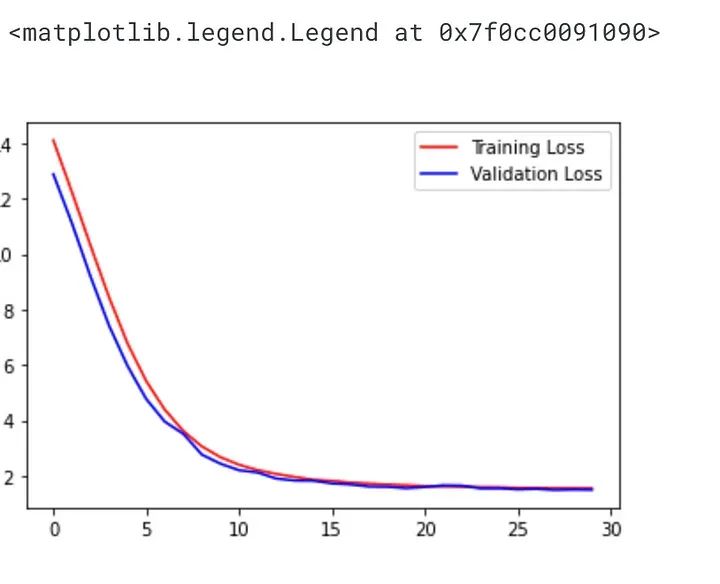
This code plots the training and validation loss of the CNN model during the training process.
The history object returned by the fit() method contains information about the training process, including the training and validation loss and accuracy for each epoch. This information can be used to visualize the model’s performance over time.
The plt.plot() function is used to plot the red training loss and the blue validation loss, with the label parameter specifying the legend label for each line. The legend() function is called to display the legend on the plot.
This code allows us to see how the model is learning, and whether it is overfitting to the training data. If the validation loss starts to increase while the training loss continues to decrease, it indicates overfitting, meaning the model is memorizing the training data rather than generalizing well to new data.
plt.plot(history.history["accuracy"] ,'r',label="Training Accuracy")
plt.plot(history.history["val_accuracy"] ,'b',label="Validation Accuracy")
plt.legend()
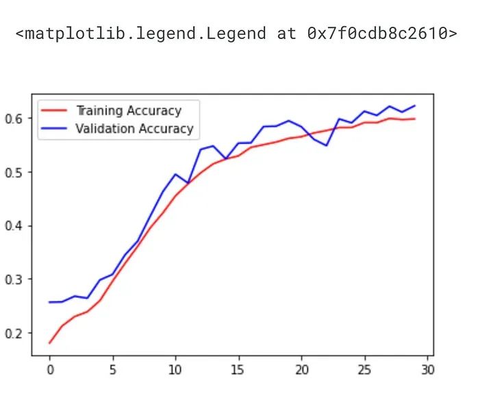
This code plots the training and validation accuracy of the CNN model during the training process.
The history object returned by the fit() method contains information about the training process, including the training and validation loss and accuracy for each epoch. This information can be used to visualize the model’s performance over time.
The plt.plot() function is used to plot the red training accuracy and the blue validation accuracy, with the label parameter specifying the legend label for each line. The legend() function is called to display the legend on the plot.
This code allows us to see how the model is learning, and whether it is overfitting to the training data. If the validation accuracy starts to decrease while the training accuracy continues to increase, it indicates overfitting, meaning the model is memorizing the training data rather than generalizing well to new data.
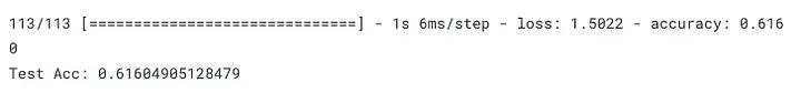
loss = model.evaluate(X_test,y_test)
print("Test Acc: " + str(loss[1]))
This code evaluates the performance of the trained CNN model on the test set.
The evaluate() method of Keras models computes the loss and metrics (as specified during model compilation) on a given test set.
The X_test and y_test arrays contain the test images and their corresponding labels, respectively. The model.evaluate() method computes the loss and accuracy of the model on the test set. The evaluate() method returns the loss value and accuracy value as an array.
The test accuracy is printed using the loss object returned by model.evaluate(). The test accuracy gives us an understanding of how well the model performs on new, unseen data.
preds = model.predict(X_test)
y_pred = np.argmax(preds , axis = 1 )
This code generates predictions for the test set using the trained CNN model.
The predict() method of Keras models generates predictions for a given input dataset X_test. In this case, the array contains the test images we want to predict.
The preds array contains the predicted probabilities for each class for each test image, where each row corresponds to a test image and each column corresponds to a class.
The np.argmax() function is used to extract the index of the class with the highest predicted probability for each test image. This gives us the predicted class labels for the test set.
The predicted class labels can then be compared with the actual class labels y_test to evaluate the model’s performance on the test set.
label_dict = {0 : 'Angry', 1 : 'Disgust', 2 : 'Fear', 3 : 'Happiness', 4 : 'Sad', 5 : 'Surprise', 6 : 'Neutral'}
figure = plt.figure(figsize=(20, 8))
for i, index in enumerate(np.random.choice(X_test.shape[0], size=24, replace=False)):
    ax = figure.add_subplot(4, 6, i + 1, xticks=[], yticks=[])
    ax.imshow(np.squeeze(X_test[index]))
    predict_index = label_dict[(y_pred[index])]
    true_index = label_dict[np.argmax(y_test,axis=1)[index]]

    ax.set_title("{} ({})".format((predict_index),
                                  (true_index)),
                                  color=("green" if predict_index == true_index else "red"))
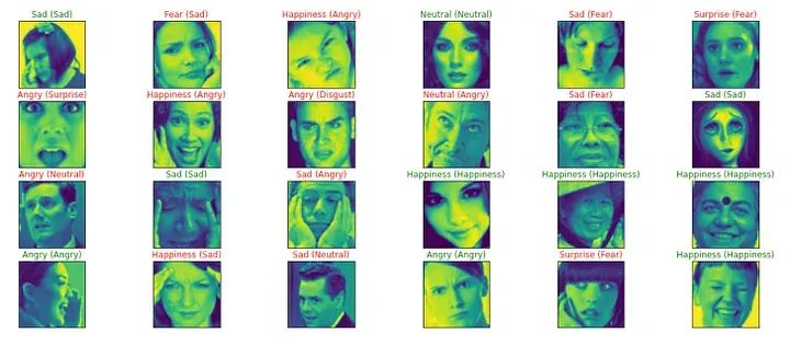
This code generates a visualization of a random subset of test images along with their true and predicted labels.
The label_dict dictionary maps the integer class labels to their corresponding string labels.
Then, the code generates a figure containing 24 subplots (4 rows, 6 columns), where each subplot displays a random test image along with its predicted and true labels. The function randomly selects 24 indices from the X_test array.
For each subplot, the imshow() function is used to display the test image, and the set_title() function displays the predicted label and true label in the title of the subplot. If the predicted label matches the true label, it is highlighted in green; otherwise, it is highlighted in red.
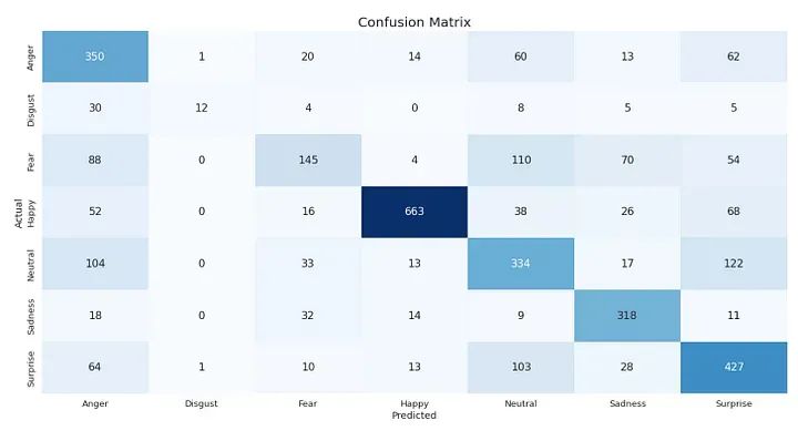
CLASS_LABELS  = ['Anger', 'Disgust', 'Fear', 'Happy', 'Neutral', 'Sadness', "Surprise"]
cm_data = confusion_matrix(np.argmax(y_test, axis = 1 ), y_pred)
cm = pd.DataFrame(cm_data, columns=CLASS_LABELS, index = CLASS_LABELS)
cm.index.name = 'Actual'
cm.columns.name = 'Predicted'
plt.figure(figsize = (15,10))
plt.title('Confusion Matrix', fontsize = 20)
sns.set(font_scale=1.2)
ax = sns.heatmap(cm, cbar=False, cmap="Blues", annot=True, annot_kws={"size": 16}, fmt='g')
This code generates a heatmap of the confusion matrix for the model’s predictions on the test set.
The CLASS_LABELS list contains the names of the seven emotion classes.
The confusion_matrix() function from the metrics module in scikit-learn is used to compute the confusion matrix for the model’s predictions on the test set. The np.argmax() function is used to convert the one-hot encoded true labels and predicted labels into integer labels.
The resulting confusion matrix is stored in a pandas DataFrame cm, with class names as row and column labels. The heatmap is then displayed using the heatmap() function from seaborn, with the values of the confusion matrix annotated and the font size increased using sns.set(font_scale=1.2).

from sklearn.metrics import classification_report
print(classification_report(np.argmax(y_test, axis = 1 ),y_pred,digits=3))
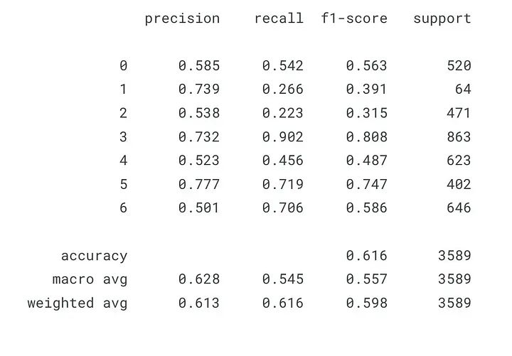
The output of classification_report() includes the following:
-
Precision: The ratio of predicted positive cases to actual positive cases. Mathematically, it is TP / (TP + FP), where TP is the number of true positives and FP is the number of false positives. A high precision score indicates that the model is accurate when predicting the positive class. -
Recall: The ratio of actual positive cases that the model correctly predicts as positive. Mathematically, it is TP / (TP + FN), where FN is the number of false negatives. A higher recall score indicates that the model is able to correctly identify positive cases. -
F1 Score: The harmonic mean of precision and recall. It considers both precision and recall and provides a single score that balances both. Mathematically, it is 2 * (precision * recall) / (precision + recall). -
Support: The number of actual occurrences of each class in the test data.
Below are the explanations for the different rows in the classification report:
-
Precision: The first row shows the precision scores for each class. -
Recall: The second row shows the recall scores for each class. -
F1 Score: The third row shows the F1 scores for each class. -
Support: The last row shows the number of occurrences of each class in the test data.
Note that the macro and weighted averages are also located at the bottom of the report.
Fine-tuning the Model
model = cnn_model()
model.compile(optimizer=tf.keras.optimizers.SGD(0.001),
                loss='categorical_crossentropy',
                metrics = ['accuracy'])
The optimizer of the model has been changed from Adam to SGD with a learning rate of 0.001. The loss function remains the same, which is categorical crossentropy. The accuracy metric is also the same.
history = model.fit(train_generator,
                    epochs=30,
                    batch_size=64,
                    verbose=1,
                    callbacks=[checkpointer],
                    validation_data=val_generator)
This code trains the model for another 30 epochs using the training and validation data from train_generator and val_generator, respectively, with a batch size of 64.
The checkpointer callback is also used to save the best model based on validation accuracy.
loss = model.evaluate(X_test,y_test)
print("Test Acc: " + str(loss[1]))
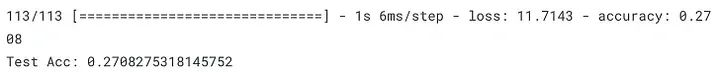
This code prints the test accuracy after fine-tuning the model using the SGD optimizer with a learning rate of 0.001.
plt.plot(history.history["loss"] ,'r', label="Training Loss")
plt.plot(history.history["val_loss"] ,'b', label="Validation Loss")
plt.legend()
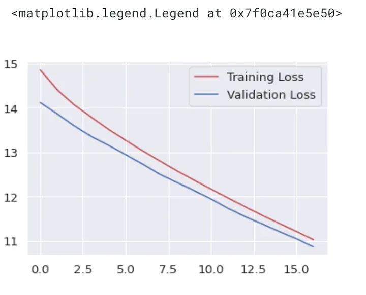
This plot shows the training loss (red) and validation loss (blue) for each epoch during the training of the model. The x-axis represents the number of epochs, and the y-axis represents the loss. It helps to determine whether the model is overfitting or underfitting.
If the training loss is decreasing while the validation loss is increasing or not decreasing, it indicates that the model is overfitting. If both training and validation losses are high, it indicates that the model is underfitting.
From the plot, it seems that both training and validation losses are decreasing, indicating that the model is learning from the data.
Change the Number of Epochs
model.compile(
    optimizer = Adam(lr=0.0001),
    loss='categorical_crossentropy',
    metrics=['accuracy'])
checkpointer = [EarlyStopping(monitor = 'val_accuracy', verbose = 1,
                              restore_best_weights=True,mode="max",patience = 10),
                              ModelCheckpoint('best_model.h5',monitor="val_accuracy",verbose=1,
                              save_best_only=True,mode="max")]
history = model.fit(train_generator,
                    epochs=50,
                    batch_size=64,
                    verbose=1,
                    callbacks=[checkpointer],
                    validation_data=val_generator)
The updated code trains the model for 50 epochs again, with early stopping callbacks set to wait for 10 epochs. The best model will be saved as “best_model.h5” with the highest validation accuracy.
The model will be compiled using the Adam optimizer with a learning rate of 0.0001, categorical crossentropy loss, and accuracy as metrics. The training generator and validation generator are defined earlier using data augmentation techniques.
loss = model.evaluate(X_test,y_test)
print("Test Acc: " + str(loss[1]))
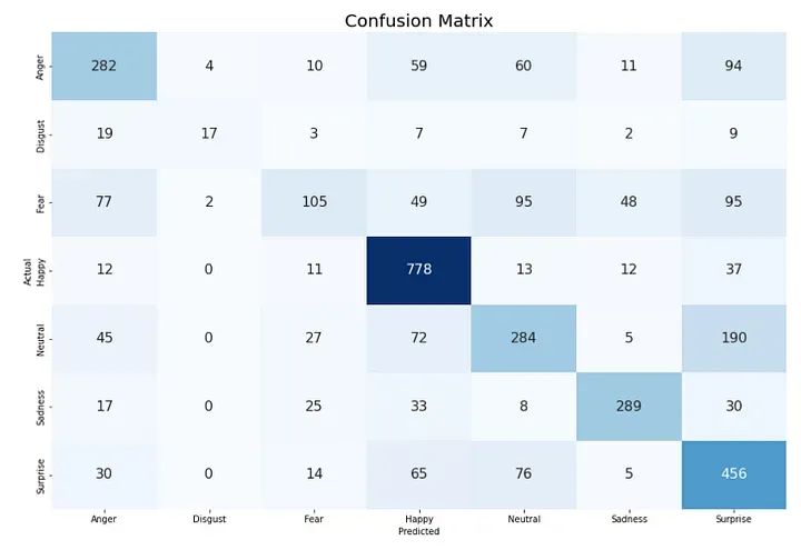
CLASS_LABELS  = ['Anger', 'Disgust', 'Fear', 'Happy', 'Neutral', 'Sadness', "Surprise"]
cm_data = confusion_matrix(np.argmax(y_test, axis = 1 ), y_pred)
cm = pd.DataFrame(cm_data, columns=CLASS_LABELS, index = CLASS_LABELS)
cm.index.name = 'Actual'
cm.columns.name = 'Predicted'
plt.figure(figsize = (20,10))
plt.title('Confusion Matrix', fontsize = 20)
sns.set(font_scale=1.2)
ax = sns.heatmap(cm, cbar=False, cmap="Blues", annot=True, annot_kws={"size": 16}, fmt='g')
Download 1: OpenCV-Contrib Extension Module Chinese Version Tutorial

Reply "Extension Module Chinese Tutorial" in the backend of "Beginner Learning Visuals" public account to download the first Chinese version of the OpenCV extension module tutorial available online, covering over twenty chapters including extension module installation, SFM algorithms, stereo vision, target tracking, biological vision, super-resolution processing, etc.

Download 2: Python Visual Practical Project 52 Lectures

Reply "Python Visual Practical Project" in the backend of "Beginner Learning Visuals" public account to download 31 visual practical projects including image segmentation, mask detection, lane line detection, vehicle counting, eyeliner addition, license plate recognition, character recognition, emotion detection, text content extraction, facial recognition, etc., to help quickly learn computer vision.

Download 3: OpenCV Practical Project 20 Lectures

Reply "OpenCV Practical Project 20 Lectures" in the backend of "Beginner Learning Visuals" public account to download 20 practical projects based on OpenCV, achieving advanced learning of OpenCV.

Group Chat

Welcome to join the reader group of the public account to communicate with peers. Currently, there are WeChat groups for SLAM, 3D vision, sensors, autonomous driving, computational photography, detection, segmentation, recognition, medical imaging, GAN, algorithm competitions, etc. (will be gradually subdivided in the future). Please scan the WeChat ID below to join the group, with the note: "Nickname + School/Company + Research Direction", for example: "Zhang San + Shanghai Jiao Tong University + Visual SLAM". Please follow the format for notes, otherwise, you will not be approved. After successfully adding, you will be invited to relevant WeChat groups based on your research direction. Please do not send advertisements in the group, otherwise, you will be removed, thank you for your understanding~