Understanding Common Machine Learning Models

Click on the above“Beginner Learning Vision” to select “Star” or “Pin”

Important content delivered at the first time

Linear Models

Linear models are the simplest and most basic machine learning models. Their mathematical form is as follows: g(x;w)=. Sometimes, we also add a bias term b on top of, but as long as we expand x with a one-dimensional constant component, we can merge the linear function with a bias term into the form of. Linear models are very straightforward, and each dimension of the parameters corresponds to the importance of the corresponding feature dimension. However, it is clear that linear models also have certain limitations.

First, the range of values for linear models is unrestricted; depending on the specific values of w and x, their output can be a very large positive number or a very small negative number. However, when classifying, we expect the model output to be the probability that a sample belongs to the positive class (such as positive feedback), which is usually a probability value between 0 and 1. To bridge the gap between these two, people often use a log-odds function to transform the output of the linear model, resulting in the following formula:

After transformation, strictly speaking, g(x;w) is no longer a linear function but a nonlinear function derived from a linear function, which we usually refer to as a generalized linear function. The log-odds model itself is a probabilistic form, very suitable for training using log-likelihood loss or cross-entropy loss.

Secondly, linear models can only explore linear combinations of features and cannot model more complex and powerful nonlinear combinations. To address this issue, we can perform some explicit nonlinear pre-transformations on the input features (such as exponential, logarithmic, polynomial transformations of one-dimensional features, and cross products of multi-dimensional features), or use kernel methods to implicitly map the original feature space to a high-dimensional nonlinear space and then construct linear models in that high-dimensional space.

Kernel Methods and Support Vector Machines

The basic idea of kernel methods is to map the input data to a high-dimensional Hilbert space through a nonlinear transformation. In this high-dimensional space, problems that are linearly inseparable in the original input space become easier to solve, or even linearly separable. Support Vector Machines (SVM) are one of the most typical kernel methods. Below, we will use support vector machines as an example to briefly introduce kernel methods.

The basic idea of support vector machines is to transform the original input space into a high-dimensional (even infinite-dimensional) space through a kernel function, and find a hyperplane in this space that can separate the positive and negative examples in the training set as much as possible (to describe it in more academic terms, it is to maximize the margin between positive and negative examples). So how can we achieve a nonlinear mapping of the space through the kernel function? Let’s start from the beginning.

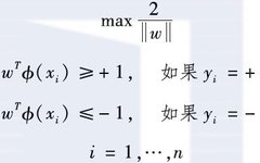
Assume there exists a nonlinear mapping function Φ that can help us transform the original input space into a high-dimensional nonlinear space. Our goal is to find a linear hyperplane in the transformed space, which can separate all positive and negative examples and maximize the margin between the closest positive and negative examples to that hyperplane. This requirement can be mathematically described as follows:

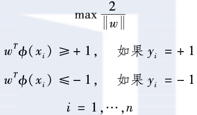
Where, is the margin between the closest positive and negative examples to the hyperplane (as shown in Figure 2.6).

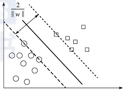
Figure 2.6 Maximizing Margin and Support Vector Machines

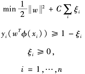
The above mathematical description is equivalent to the following optimization problem: min12w2

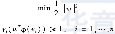
The constraints in the above equation require all positive and negative examples to be located on either side of the hyperplane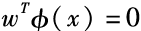. In some cases, this constraint may be too strong because the training set we have is sometimes inseparable. At this point, we need to introduce slack variables, rewriting the above optimization problem as:

In fact, this new expression is equivalent to minimizing a Hinge loss function with a regularization term added. This is because when is less than 0, the sample is correctly classified by the hyperplane, ξi=0; otherwise, ξi will be greater than 0, and is‘s upper bound: minimizing ξi thus minimizes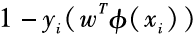. Based on the above discussion, support vector machines actually minimize the following objective function:

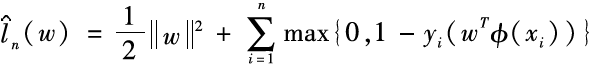
Where, is the regularization term, and minimizing it can restrict the model space, effectively improving the model’s generalization ability (which means making the model’s performance on the training set and the test set closer).

To solve the aforementioned constrained optimization problem, a common technique is to use the Lagrange multiplier method to convert it into a dual problem for solving. Specifically, the dual problem corresponding to support vector machines is as follows:

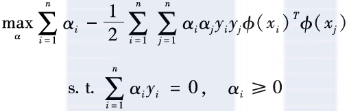
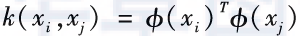
In the dual space, the description of this optimization problem only relates to the inner product of and and is unrelated to the specific form of the mapping function. Therefore, we only need to define the kernel function k(xi,xj) between two samples and to represent their inner product after being mapped to the high-dimensional space:

At this point, we have clarified how the kernel function relates to the space transformation. There can be many different choices for kernel functions; Table 2.1 lists several commonly used kernel functions.

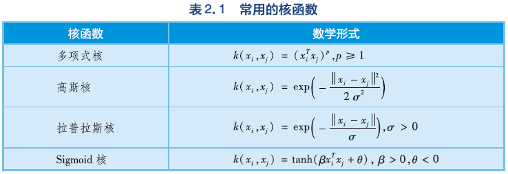
In fact, as long as a symmetric function corresponds to a kernel matrix that satisfies the positive semi-definite condition, it can be used as a kernel function, and there will always be a corresponding space mapping. In other words, any kernel function implicitly defines a Reproducing Kernel Hilbert Space (RKHS). In this space, the inner product of two vectors equals the value of the corresponding kernel function.

Decision Trees and Boosting

Decision trees are also a common type of machine learning model. Their basic idea is to construct a tree-structured decision model based on the attributes of the data. A decision tree consists of a root node, several internal nodes, and several leaf nodes. Leaf nodes correspond to the final decision results, while other nodes make judgments and branches based on a certain attribute of the data: at such nodes, a certain attribute (feature) of the data is tested, and based on the test results, the sample is divided into a certain subtree of that node. Through the decision tree, we can start from the root node and ultimately assign a specific sample to a certain leaf node, achieving the corresponding prediction function.

Because the branching operation at each node is nonlinear, decision trees can implement relatively complex nonlinear mappings. The goal of decision tree algorithms is to learn a decision tree with strong generalization ability from the training data, meaning it can accurately classify unknown samples into the correct leaf nodes. To achieve this goal, the decision tree we construct during the training process should not be too complex; otherwise, it may overfit the training data and fail to properly handle unknown test data. Common decision tree algorithms include Classification and Regression Trees (CART), ID3 algorithm, C4.5 algorithm, and Decision Stump, among others. The basic processes of these algorithms are quite similar, including two fundamental steps: partition selection and pruning.

The partition selection problem is how to divide the samples in a dataset at a certain node based on certain criteria into a subtree. Common criteria include information gain, gain ratio, and Gini index. Although their specific mathematical forms differ, the core ideas are similar. Here, we will introduce information gain as an example. Information gain refers to the degree of purity improvement of the sample set obtained by partitioning the dataset D using feature j at a certain node. The specific mathematical definition of information gain is as follows:

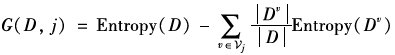
Where, is the value set of feature, and is the subset of samples whose feature takes the value. Entropy(D) is the information entropy of the sample set D, which describes the distribution of samples from different categories within D. The more evenly the samples from different categories are distributed, the larger the information entropy, and the lower the purity of the set; conversely, the more concentrated the sample distribution, the smaller the information entropy, and the higher the purity of the set. The goal of sample partitioning is to find the feature that minimizes the average information entropy after partitioning, thereby maximizing information gain.

The pruning process aims to suppress overfitting. If the decision tree is very complex, with each leaf node corresponding to only one training sample, it can achieve maximum information gain, but this will lead to overfitting the training data, resulting in a loss of accuracy on the test data. To address this issue, pruning operations can be used to reduce the complexity of the decision tree. Pruning can be divided into pre-pruning and post-pruning: pre-pruning refers to estimating each node before partitioning during the decision tree generation process. If the current node’s partition does not improve the generalization performance of the decision tree (which can usually be assessed using a cross-validation set), then the partition is stopped, and the current node is marked as a leaf node; post-pruning refers to first generating a complete decision tree from the training set and then examining whether removing each node (i.e., merging that node and its subtree into a leaf node) improves generalization capability from the bottom up. If there is an improvement, pruning is performed.

In some cases, due to the difficulty of the learning task, the performance of a single decision tree may be limited. In such cases, people often use ensemble learning to enhance the final learning ability. There are many methods for ensemble learning, such as Bagging and Boosting. The basic idea of Boosting is to first train a weak learner, and then adjust the distribution of training samples based on the performance of the weak learner so that the previously misclassified samples receive more attention in subsequent learning, and then train the next weak learner based on the adjusted sample distribution. This process continues until the number of weak learners reaches a preset limit or the weighted combination of weak learners achieves the desired accuracy. The final predictive model is the weighted sum of all these weak learners:

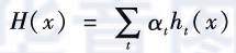
Where, is the weight coefficient, which can be obtained during the training process according to the accuracy of the current weak learner using empirical formulas, or can be obtained after the training process ends (after all weak learners have been trained) using new learning objectives through additional optimization methods.

Research has shown that Boosting performs very well in resisting overfitting, meaning that as the training process progresses, even if the error on the training set has been reduced to 0, more iterations can still improve the model’s performance on the test set. This phenomenon is explained by the Margin Theory: as the iterations continue, although the error on the training set no longer changes, the classification confidence of the training samples (corresponding to the margin at each sample point) continues to increase. To this day, Boosting algorithms, especially those combined with decision trees such as Gradient Boosting Decision Trees (GBDT), remain the backbone of many practical applications and are popular in data mining competitions.

Neural Networks

Neural networks are a typical class of nonlinear models, inspired by biological neural networks. Through studies of the biological mechanisms of the brain, it has been found that the basic unit is the neuron, where each neuron receives input signals from upstream neurons through dendrites, processes these signals, and then transmits the output signals to downstream neurons through axons. When the total input signal to a neuron reaches a certain intensity, it activates an output signal; otherwise, there is no output signal (as shown in Figure 2.7a).

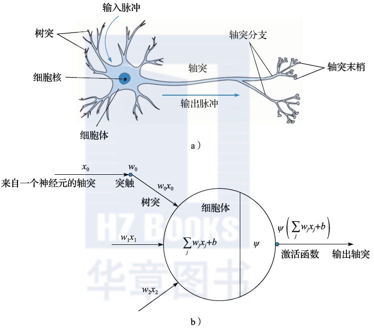
Figure 2.7 Structure of Neurons and Artificial Neural Networks

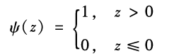
This biological principle can be expressed in mathematical language as shown in Figure 2.7b. A neuron performs a linear weighted sum of the input signals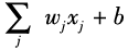, and then drives an activation function ψ based on the size of the sum to generate an output signal. The activation function in biological systems is similar to a step function:

However, because the step function itself is discontinuous, it is not a good choice for machine learning. Therefore, when designing artificial neural networks, continuous activation functions are usually used, such as the Sigmoid function, hyperbolic tangent function (tanh), and Rectified Linear Unit (ReLU). Their mathematical forms and function shapes are shown in Figure 2.8.

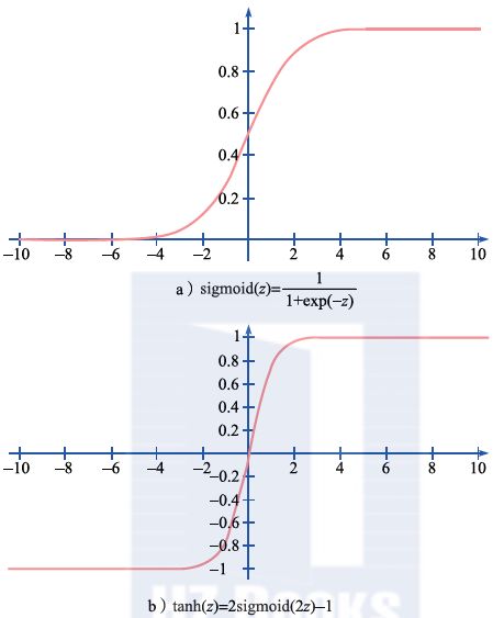
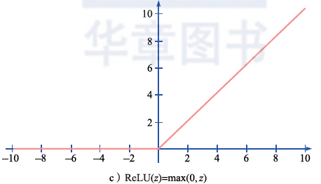
Figure 2.8 Common Activation Functions

1. Fully Connected Neural Networks

The most basic neural network connects the neurons described above together to form a hierarchical structure (as shown in Figure 2.9), which we call a fully connected neural network. In this network, the leftmost corresponds to the input nodes, the rightmost corresponds to the output nodes, and the three middle layers are hidden nodes (we refer to the corresponding layers as hidden layers). Each hidden node performs a weighted sum of the outputs from the previous layer nodes, passes through a nonlinear activation function, and outputs to the next layer. The output layer generally uses a simple linear function or further uses the softmax function to convert the output into probability form.

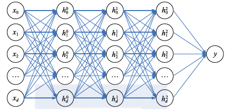
Figure 2.9 Fully Connected Neural Network

Although fully connected neural networks appear simple, they have a very powerful expressive ability. As early as the 1980s, it was proven that the famous Universal Approximation Theorem holds. The earliest Universal Approximation Theorem was proven for the Sigmoid activation function, and the general Universal Approximation Theorem was proven in 2001. Its mathematical description states that under certain conditions on the activation function, for any continuous function in a given input space and approximation accuracy ε, there exists a natural number Nε and a single hidden layer fully connected neural network with Nε hidden nodes that can approximate this continuous function with an accuracy less than ε. This theorem is very important as it tells us that fully connected neural networks can be used to solve very complex problems; when other models (such as linear models, support vector machines, etc.) cannot approximate the classification boundaries of such problems, neural networks can still perform excellently and effortlessly. In recent years, it has been pointed out that deep networks have stronger expressiveness, meaning that to express certain logical functions, deep networks require significantly fewer hidden nodes than shallow networks. This is beneficial for model storage and optimization, which has led to increased attention and usage of deeper neural networks.

Fully connected neural networks often select a cross-entropy loss function during training and use gradient descent to solve the model parameters (in practice, to reduce the cost of each model update, mini-batch stochastic gradient descent is used). It should be noted that although the cross-entropy loss is a convex function, due to the non-linear and non-convex nature of multi-layer neural networks, the loss function is actually severely non-convex regarding the model parameters. In this case, using gradient descent usually only finds local optimal solutions. To address this issue, techniques such as multiple random initializations or simulated annealing are often used in practice to find better solutions in a global sense. Recent studies have shown that under certain conditions, if the neural network is sufficiently deep, all its local optimal solutions actually have loss function values very similar to the global optimal solution. In other words, for deep neural networks, the concern that “only local optimal solutions can be found” is not necessarily a fatal flaw; in many cases, this local optimal solution is already good enough to achieve very good actual prediction accuracy.

In addition to concerns about local and global optimal solutions, there are actually two other difficulties in using deep neural networks.

• First, because deep neural networks have very strong expressive power, they can easily overfit the training data, leading to poor performance on the test data. To solve this problem, many methods have been proposed, including DropOut, Data Augmentation, Batch Normalization, Weight Decay, and Early Stopping, which introduce randomness, pseudo-training samples, or limit the model space to improve the model’s generalization ability.

• Second, when the network is very deep, the prediction error at the output layer is difficult to smoothly propagate back through the layers, making it difficult for those hidden layers close to the input layer to receive adequate training. This problem is also known as the “vanishing gradient problem.” Research has shown that the vanishing gradient problem is mainly caused by the non-linear activation functions of neural networks, as the derivatives of non-linear activation functions are not large. When using gradient descent for optimization, the product of the derivatives of non-linear activation functions appears in the gradient calculation formula, leading to a gradual decrease in the gradient’s magnitude through the layers. To address this issue, linear connections or linear paths controlled by gate circuits have been introduced between layers to facilitate the smooth backpropagation of gradient information.

2. Convolutional Neural Networks

In addition to fully connected neural networks, Convolutional Neural Networks (CNN) are also a very commonly used network structure, especially suitable for processing image data.

The design of convolutional neural networks is inspired by the biological visual system. Research has shown that each visual cell is only sensitive to a small local area, and a large number of visual cells are tiled across the field of vision, which can effectively utilize the spatial local correlation of natural images. Similarly, convolutional neural networks introduce the concept of local connectivity and tile filters (also known as convolutional kernels) with the same parameter structure spatially. These filters have large overlapping areas, equivalent to a spatial sliding window, which analyzes the information within the window using the same filter as it slides to different spatial positions. Thus, although the network is large, the number of model parameters is not many due to the sharing of parameters across different positions, resulting in high parameter efficiency.

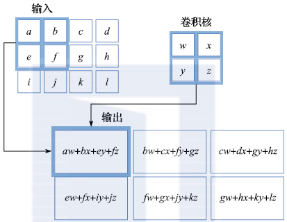
Figure 2.10 Illustration of the Convolution Process

In addition to convolution, pooling is also an important component of convolutional neural networks. The purpose of pooling is to compress the original feature map, better reflecting the translation invariance of image recognition and effectively expanding the receptive field of subsequent convolution operations. Pooling is generally not a parameterized module, unlike convolution, but rather uses deterministic methods to calculate the average, median, maximum, or minimum of local areas (in recent years, some scholars have also begun to study parameterized pooling operators). Figure 2.11 describes the effect of performing 2×2 max pooling on a local area of an image.

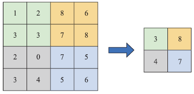
Figure 2.11 Illustration of the Pooling Operation

In practice, multiple convolutional layers and pooling layers can be alternately connected to continuously extract high-level semantic features from the original image. After this, a fully connected network can be concatenated to perform pattern recognition or prediction based on these high-level semantic features. This process is illustrated in Figure 2.12.

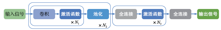
Figure 2.12 Multi-layer Convolutional Neural Network (N1, N2, N3 represent the number of repetitions of corresponding units)

In practice, people have begun to try using deeper convolutional neural networks to achieve better image classification results. Figure 2.13 describes the process of continuously refreshing the error rate on the ImageNet dataset by increasing the depth of the network in recent years. Among them, the ResNet network with 152 layers from Microsoft Research in 2015 achieved a Top-5 error rate as low as 3.57% on the ImageNet dataset, surpassing the image recognition ability of ordinary humans on specific tasks.

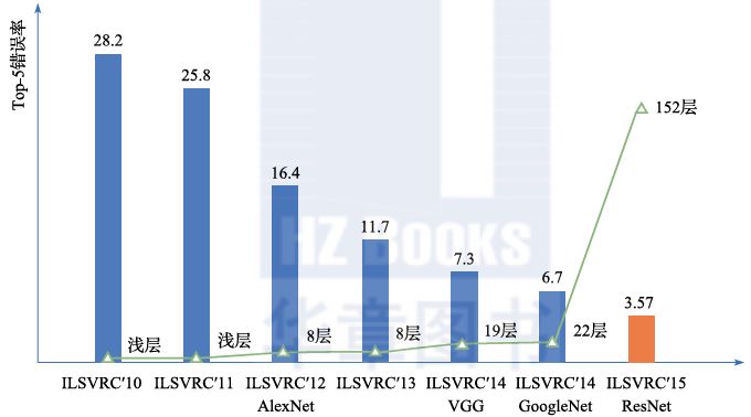
Figure 2.13 Convolutional Neural Networks Continuously Refreshing Recognition Results on the ImageNet Dataset

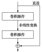
Figure 2.14 Residual Learning

As convolutional neural networks become deeper, the previously mentioned vanishing gradient problem becomes more pronounced, making training the model very difficult. To address this issue, a series of methods have been proposed in recent years, including residual learning (as shown in Figure 2.14) and densely connected networks (as shown in Figure 2.15). Experiments have shown that these methods can effectively transmit training errors to areas close to the input layer, laying a solid practical foundation for training deep convolutional neural networks.

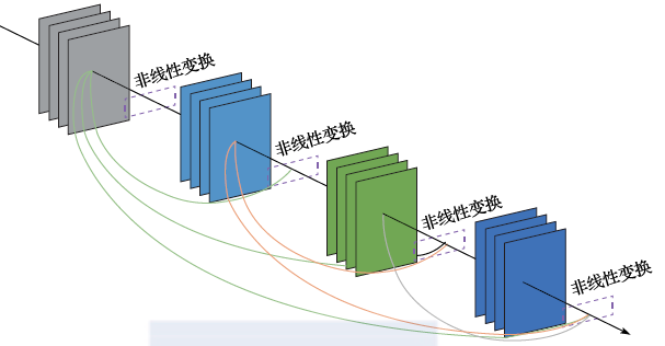
Figure 2.15 Dense Networks

3. Recurrent Neural Networks

Recurrent Neural Networks (RNN) are also designed with a strong biomimetic foundation. We can think about how we read books and newspapers. When we read a sentence, we do not simply understand the character we see at that moment; rather, the text we read previously forms a memory in our minds, and this memory helps us better understand the current text. This process is recursive; when we look at the next character, the current character and historical memory become our new memory and help us understand the next character. In fact, the design of recurrent neural networks is based on this idea. 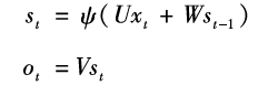We use to represent the memory at time, which is jointly influenced by the input seen at time t and the memory at time t-1. This process can be expressed by the following equation:

Clearly, this formula embodies the circular iteration of the memory unit. In practical applications, infinite long-term circular iterations are not very meaningful. For example, the average length of each sentence we read may only be a dozen characters. Therefore, we can completely unfold the recurrent neural network in the time domain and use gradient descent to obtain the parameter matrices U, W, and V on the unfolded network, as shown in Figure 2.16. In the terminology of recurrent neural networks, we call this Back Propagation Through Time (BPTT).

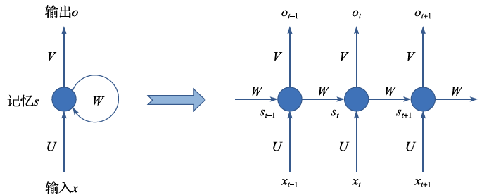
Figure 2.16 Unfolding of Recurrent Neural Networks

Similar to fully connected neural networks and convolutional neural networks, when the recurrent neural network is unfolded in the time domain, it also encounters the vanishing gradient problem. To address this issue, a method relying on gate circuits to control the flow of information has been proposed. In other words, there are both linear and nonlinear paths between two layers of the recurrent neural network, and which path is open or closed, or to what extent, is controlled by a group of gate circuits. This gate circuit is also parameterized, and these parameters are learnable during the optimization process of the neural network. Two well-known methods are LSTM and GRU (as shown in Figure 2.17). GRU is simpler than LSTM, which has three gate circuits (input gate, forget gate, output gate), while GRU has two (reset gate, update gate). The effects of both in practice are similar, but GRU tends to train faster, thus becoming more popular in recent years.

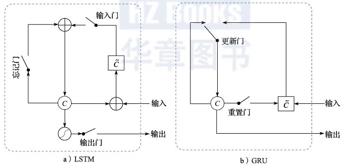
Figure 2.17 Gate Circuits in Recurrent Neural Networks

Recurrent neural networks can effectively model time series. Based on the different situations of the sequences they process, the application scenarios of recurrent neural networks can be divided into point-to-sequence, sequence-to-point, and sequence-to-sequence types (as shown in Figure 2.18).

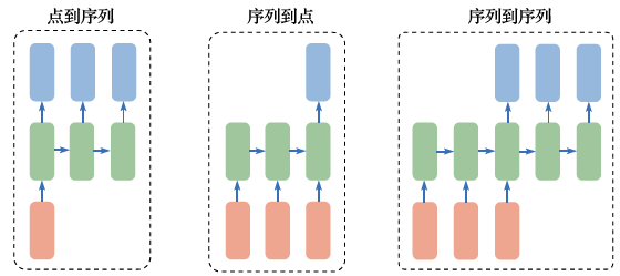
Figure 2.18 Different Applications of Recurrent Neural Networks

Next, we will introduce several application scenarios of recurrent neural networks.

(1) Image Captioning: Point-to-Sequence Application of Recurrent Neural Networks

In this application, the input is the encoded information of an image (which can be obtained through the intermediate layers of a convolutional neural network or directly using the category labels predicted by the convolutional neural network), and the output is a natural language text generated by the recurrent neural network to describe the content of that image.

(2) Sentiment Classification: Sequence-to-Point Application of Recurrent Neural Networks

In this application, the input is a segment of text information (a time sequence), and the output is the sentiment classification label (positive or negative sentiment). The recurrent neural network is used to analyze the input text, and its hidden nodes contain the encoding information of the entire input statement, which is then mapped to the appropriate sentiment category through a fully connected classifier.

(3) Machine Translation: Sequence-to-Sequence Application of Recurrent Neural Networks

In this application, the input is a text in one language (a time sequence), and the output is a text in another language (a time sequence). The recurrent neural network is used twice in this application: the first time to analyze and encode the input source language text, and the second time to utilize this encoding information to drive the output of a segment of text in the target language.

When using sequence-to-sequence recurrent neural networks for machine translation, a problem arises in practice. The degree of dependence of a certain word in the output translation result on various words in the input is different. Encoding the entire input sentence into a vector to drive the output sentence leads to overly coarse information granularity or neglects long-range dependencies. To solve this problem, people have introduced the so-called “attention mechanism” based on the standard sequence-to-sequence recurrent neural networks. With its help, the generation of each word at the output leverages the encoding information of different words in the input. This attention mechanism is also parameterized and can automatically learn during the training process of the entire recurrent neural network.

Neural networks, especially deep neural networks, are a rapidly developing research area. With continuous attention from both academia and industry, this field has gained more development opportunities than other machine learning fields, with new network structures or optimization methods being continuously proposed. If readers are interested in this field, please pay attention to the latest papers published at mainstream academic conferences on machine learning every year.

References

[1] Cao Z, Qin T, Liu T Y, et al. Learning to Rank: From Pairwise Approach to Listwise Approach[C]//Proceedings of the 24th international conference on Machine learning. ACM, 2007: 129-136.

[2] Liu T Y. Learning to rank for information retrieval[J]. Foundations and Trends in Information Retrieval, 2009, 3(3): 225-331.

[3] Kotsiantis S B, Zaharakis I, Pintelas P. Supervised Machine Learning: A Review of Classification Techniques[J]. Emerging Artificial Intelligence Applications in Computer Engineering, 2007, 160: 3-24.

[4] Chapelle O, Scholkopf B, Zien A. Semi-supervised Learning (chapelle, o. et al., eds.; 2006)[J]. IEEE Transactions on Neural Networks, 2009, 20(3): 542-542.

[5] He D, Xia Y, Qin T, et al. Dual learning for machine translation[C]//Advances in Neural Information Processing Systems. 2016: 820-828.

[6] Hastie T, Tibshirani R, Friedman J. Unsupervised Learning[M]//The Elements of Statistical Learning. New York: Springer, 2009: 485-585.

[7] Sutton R S, Barto A G. Reinforcement Learning: An Introduction[M]. Cambridge: MIT press, 1998.

[8] Seber G A F, Lee A J. Linear Regression Analysis[M]. John Wiley & Sons, 2012.

[9] Harrell F E. Ordinal Logistic Regression[M]//Regression modeling strategies. New York: Springer, 2001: 331-343.

[10] Cortes C, Vapnik V. Support-Vector Networks[J]. Machine Learning, 1995, 20(3): 273-297.

[11] Quinlan J R. Induction of Decision Trees[J]. Machine Learning, 1986, 1(1): 81-106.

[12] McCulloch, Warren; Walter Pitts (1943). “A Logical Calculus of Ideas Immanent in Nervous Activity” [EB]. Bulletin of Mathematical Biophysics. 5(4): 115-133.

[13] LeCun Y, Jackel L D, Bottou L, et al. Learning Algorithms for Classification: A Comparison on Handwritten Digit Recognition[J]. Neural networks: The Statistical Mechanics Perspective, 1995, 261: 276.

[14] Elman J L. Finding structure in time[J]. Cognitive Science, 1990, 14(2): 179-211.

[15] Zhou Zhihua. Machine Learning[M]. Beijing: Tsinghua University Press, 2017.

[16] Tom Mitchell. Machine Learning[M]. McGraw-Hill, 1997.

[17] Nasrabadi N M. Pattern Recognition and Machine Learning[J]. Journal of Electronic Imaging, 2007, 16(4): 049901.

[18] Voorhees E M. The TREC-8 Question Answering Track Report[C]//Trec. 1999, 99: 77-82.

[19] Wang Y, Wang L, Li Y, et al. A Theoretical Analysis of Ndcg Type Ranking Measures[C]//Conference on Learning Theory. 2013: 25-54.

[20] Devroye L, Györfi L, Lugosi G. A Probabilistic Theory of Pattern Recognition[M]. Springer Science & Business Media, 2013.

[21] Breiman L, Friedman J, Olshen R A, et al. Classification and Regression Trees[J]. 1984.

[22] Quinlan J R. C4. 5: Programs for Machine Learning[M]. Morgan Kaufmann, 1993.

[23] Iba W, Langley P. Induction of One-level Decision Trees[J]//Machine Learning Proceedings 1992. 1992: 233-240.

[24] Breiman L. Bagging predictors[J]. Machine Learning, 1996, 24(2): 123-140.

[25] Schapire R E. The Strength of Weak Learnability[J]. Machine Learning, 1990, 5(2): 197-227.

[26] Schapire R E, Freund Y, Bartlett P, et al. Boosting the Margin: A New Explanation for The Effectiveness of Voting Methods[J]. Annals of Statistics, 1998: 1651-1686.

[27] Friedman J H. Greedy Function Approximation: A Gradient Boosting Machine[J]. Annals of statistics, 2001: 1189-1232.

[28] Gybenko G. Approximation by Superposition of Sigmoidal Functions[J]. Mathematics of Control, Signals and Systems, 1989, 2(4): 303-314.

[29] Csáji B C. Approximation with Artificial Neural Networks[J]. Faculty of Sciences, Etvs Lornd University, Hungary, 2001, 24: 48.

[30] Sun S, Chen W, Wang L, et al. On the Depth of Deep Neural Networks: A Theoretical View[C]//AAAI. 2016: 2066-2072.

[31] Kawaguchi K. Deep Learning Without Poor Local Minima[C]//Advances in Neural Information Processing Systems. 2016: 586-594.

[32] Srivastava N, Hinton G, Krizhevsky A, et al. Dropout: A Simple Way to Prevent Neural Networks from Overfitting[J]. The Journal of Machine Learning Research, 2014, 15(1): 1929-1958.

[33] Tanner M A, Wong W H. The Calculation of Posterior Distributions by Data Augmentation[J]. Journal of the American statistical Association, 1987, 82(398): 528-540.

[34] Ioffe S, Szegedy C. Batch Normalization: Accelerating Deep Network Training by Reducing Internal Covariate Shift[C]//International Conference on Machine Learning. 2015: 448-456.

[35] Krogh A, Hertz J A. A Simple Weight Decay Can Improve Generalization[C]//Advances in neural information processing systems. 1992: 950-957.

[36] Prechelt L. Automatic Early Stopping Using Cross Validation: Quantifying the Criteria[J]. Neural Networks, 1998, 11(4): 761-767.

[37] Bengio Y, Simard P, Frasconi P. Learning Long-term Dependencies with Gradient Descent is Difficult[J]. IEEE Transactions on Neural Networks, 1994, 5(2): 157-166.

[38] Srivastava R K, Greff K, Schmidhuber J. Highway networks[J]. arXiv preprint arXiv:1505.00387, 2015.

[39] Lin M, Chen Q, Yan S. Network in Network[J]. arXiv preprint arXiv:1312.4400, 2013.

[40] He K, Zhang X, Ren S, et al. Deep Residual Learning for Image Recognition[C]//Proceedings of the IEEE Conference on Computer Vision and Pattern Recognition. 2016: 770-778.

[41] He K, Zhang X, Ren S, et al. Identity Mappings in Deep Residual Networks[C]//European Conference on Computer Vision. Springer, 2016: 630-645.

[42] Huang G, Liu Z, Weinberger K Q, et al. Densely Connected Convolutional Networks[C]//Proceedings of the IEEE Conference on Computer Vision and Pattern Recognition. 2017, 1(2): 3.

[43] Hochreiter S, Schmidhuber J. Long Short-term Memory[J]. Neural Computation, 1997, 9(8): 1735-1780.

[44] Cho K, Van Merriënboer B, Gulcehre C, et al. Learning Phrase Representations Using RNN Encoder-decoder for Statistical Machine Translation[J]. arXiv preprint arXiv:1406.1078, 2014.

[45] Cauchy A. Méthode générale pour la résolution des systemes d’équations simultanées[J]. Comp. Rend. Sci. Paris, 1847, 25(1847): 536-538.

[46] Hestenes M R, Stiefel E. Methods of Conjugate Gradients for Solving Linear Systems[M]. Washington, DC: NBS, 1952.

[47] Wright S J. Coordinate Descent Algorithms[J]. Mathematical Programming, 2015, 151(1): 3-34.

[48] Polyak B T. Newton’s Method and Its Use in Optimization[J]. European Journal of Operational Research, 2007, 181(3): 1086-1096.

[49] Dennis, Jr J E, Moré J J. Quasi-Newton Methods, Motivation and Theory[J]. SIAM Review, 1977, 19(1): 46-89.

[50] Frank M, Wolfe P. An Algorithm for Quadratic Programming[J]. Naval Research Logistics (NRL), 1956, 3(1-2): 95-110.

[51] Nesterov, Yurii. A method of solving a convex programming problem with convergence rate O (1/k2)[J]. Soviet Mathematics Doklady, 1983, 27(2).

[52] Karmarkar N. A New Polynomial-time Algorithm for Linear Programming[C]//Proceedings of the Sixteenth Annual ACM Symposium on Theory of Computing. ACM, 1984: 302-311.

[53] Geoffrion A M. Duality in Nonlinear Programming: A Simplified Applications-oriented Development[J]. SIAM Review, 1971, 13(1): 1-37.

[54] Johnson R, Zhang T. Accelerating Stochastic Gradient Descent Using Predictive Variance Reduction[C]//Advances in Neural Information Processing Systems. 2013: 315-323.

[55] Sutskever I, Martens J, Dahl G, et al. On the Importance of Initialization and Momentum in Deep Learning[C]//International Conference on Machine Learning. 2013: 1139-1147.

[56] Duchi J, Hazan E, Singer Y. Adaptive Subgradient Methods for Online Learning and Stochastic Optimization[J]. Journal of Machine Learning Research, 2011, 12(7): 2121-2159.

[57] Tieleman T, Hinton G. Lecture 6.5-rmsprop: Divide the Gradient By a Running Average of Its Recent Magnitude[J]. COURSERA: Neural networks for machine learning, 2012, 4(2): 26-31.

[58] Zeiler M D. ADADELTA: An Adaptive Learning Rate Method[J]. arXiv preprint arXiv:1212.5701, 2012.

[59] Kingma D P, Ba J. Adam: A Method for Stochastic Optimization[J]. arXiv preprint arXiv:1412.6980, 2014.

[60] Reddi S, Kale S, Kumar S. On the Convergence of Adam and Beyond[C]// International Conference on Learning Representations, 2018.

[61] Hazan E, Levy K Y, Shalev-Shwartz S. On Graduated Optimization for Stochastic Non-convex Problems[C]//International Conference on Machine Learning. 2016: 1833-1841.

Good news!
Beginner Learning Vision Knowledge Circle
Is now open to the public👇👇👇




Download 1: OpenCV-Contrib Extension Module Chinese Version Tutorial
Reply "Extension Module Chinese Tutorial" in the backend of the "Beginner Learning Vision" public account to download the first OpenCV extension module tutorial in Chinese on the internet, covering installation of extension modules, SFM algorithms, stereo vision, target tracking, biological vision, super-resolution processing, etc., with more than 20 chapters of content.

Download 2: Python Vision Practical Project 52 Lectures
Reply "Python Vision Practical Project" in the backend of the "Beginner Learning Vision" public account to download 31 vision practical projects including image segmentation, mask detection, lane line detection, vehicle counting, eyeliner addition, license plate recognition, character recognition, emotion detection, text content extraction, facial recognition, etc., to help quickly learn computer vision.

Download 3: OpenCV Practical Project 20 Lectures
Reply "OpenCV Practical Project 20 Lectures" in the backend of the "Beginner Learning Vision" public account to download 20 practical projects based on OpenCV, achieving advanced learning of OpenCV.

Group Chat

You are welcome to join the reader group of the public account to communicate with peers. Currently, there are WeChat groups for SLAM, 3D vision, sensors, autonomous driving, computational photography, detection, segmentation, recognition, medical imaging, GAN, algorithm competitions, etc. (will gradually be subdivided in the future). Please scan the WeChat number below to join the group, and note: "Nickname + School/Company + Research Direction", for example: "Zhang San + Shanghai Jiao Tong University + Vision SLAM". Please follow the format; otherwise, you will not be approved. After successful addition, you will be invited to the relevant WeChat group based on your research direction. Please do not send advertisements in the group; otherwise, you will be asked to leave the group. Thank you for your understanding~