Understanding Attention, Transformer, and BERT Principles

1. Introduction

There are countless good articles online about this topic, all of which are very detailed. The reason I am writing this blog today is firstly to deepen my understanding of this knowledge, secondly, I hope the blog content can focus more on some details that are hard to understand for new students like myself, and thirdly, to express some of my thoughts and hope to communicate with more people. The main content of this article is not a detailed description of the principles but aims to help those who have a general understanding of the principles but still feel somewhat confused. Therefore, the content is inclined towards parts that may seem simple to experts but may be unclear to those just starting with NLP. I hope that those who are destined to see this will generously teach me.

2. Detailed Explanation of Attention Principles

1. Overview

Before starting with Attention, I hope everyone is familiar with the RNN series network structures. If anyone is unclear, they can refer to my previous blog post on the principles of RNN, LSTM, and GRU, which clearly describes the network structure and forward-backward propagation process of RNN. The main reason is that although Attention has developed to the point where it is no longer limited to the NLP field and has shone in the CV field and others, it is also to make this blog easier for everyone to understand this part. From what I know, the earliest application of Attention was proposed by Google to improve the machine translation effects of the seq2seq architecture, and the encoding and decoding stages of seq2seq also use RNN series algorithms. Therefore, having a clear understanding of the RNN series is very significant for understanding the principles of Attention, which in turn aids in understanding the Transformer family. Personally, I guess many friends who have just started out still feel somewhat confused after reading others’ articles due to knowledge gaps.

2. Principles of Attention Structure

First, here is a paper that describes Attention in detail; please click here. I believe this paper contains detailed calculation formulas. Of course, this paper also proposes many improvements to the Attention mechanism, which are worth a careful read for those who can. There is also a paper published in ICRL; please click here. This paper was published earlier than the previous one and should be considered one of the earliest papers proposing the Attention mechanism. Similarly, students who can should read it closely. Before officially starting, I want to say a few more words, even though it may seem a bit redundant, but I think it is necessary to elaborate a bit more. Friends with a clear understanding of RNN algorithms know that one of the serious drawbacks of RNN is the long-term dependency problem. Although later variants like LSTM have emerged to alleviate this issue, when the sequence is very long, the LSTM in the decoding stage cannot effectively decode the earliest input sequence. Based on this, the Attention mechanism was proposed. If you are not too clear about RNN, I suggest you look at my previous blog. Next, we will enter this part’s theme. This article will also describe the algorithm principles using Attention in seq2seq applications. For the seq2seq part, some understanding is required. In simple terms, seq2seq is about transforming known input through a model to obtain the desired output. Interestingly, deep learning can indeed achieve this. First, let’s look at the seq2seq model without Attention:

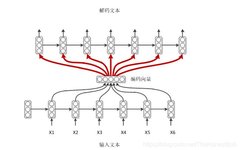
We know that both encoding and decoding use RNN, and in the encoding phase, besides the hidden layer output from the previous moment, there is also the current input character, while in the decoding phase, there is no such input. A more direct way is to use the encoding vector obtained from the encoding side as the input feature for each moment of the decoding model.Of course, if the encoder chooses LSTM, the final semantic vector C can also be used directly as input.From the diagram, we can see that the encoding vectors are equally weighted inputs, meaning that the encoding vector input at each moment is the same.The following diagram shows a seq2seq model that applies the Attention mechanism:

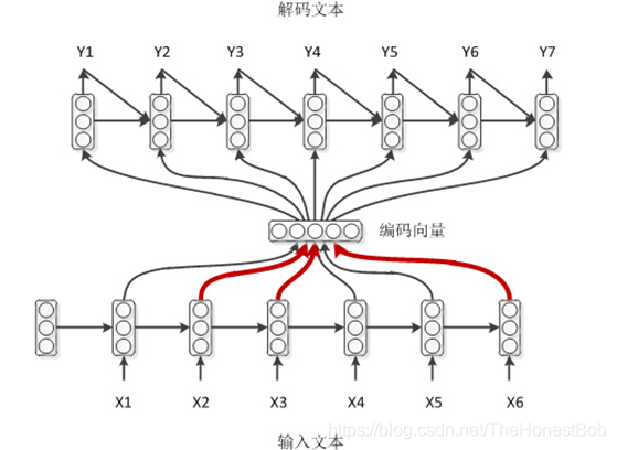
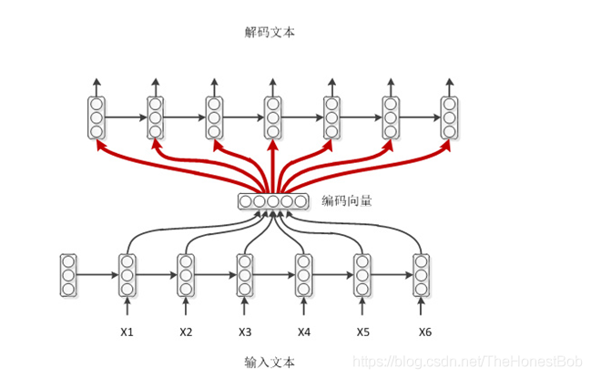
From this diagram, we can see that the input encoding vectors during the decoding phase are weighted inputs, and the weights of these encoding vectors change dynamically according to different decoding moments. Of course, besides the encoding vector input, there is also the hidden layer output from the previous moment of decoding.and the final output, where needs embedding. During training, it is the real value; during prediction, it is the predicted value. Of course, improvements can also be made here. In the TensorFlow source code, the method used is the one in the paper. This involves knowledge of seq2seq, which will not be elaborated here.Thus, the principle of Attention is quite simple, which is to obtain a specific encoding vector for different decoding moments during decoding(this sentence, though convoluted, is very important), and the most crucial part of this process is the weight of each hidden layer outputand how to calculate that weightLet’s take a look at the implementation process.First, here is the formula: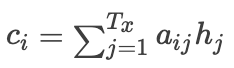Where i represents the decoding moment, represents the j-th moment in the encoding stage, represents the time step in the encoding phase.Then, represents the weight of the j-th encoding hidden layer at the i-th decoding moment.This formula illustrates how the input encoding vector at the i-th decoding moment is obtained, and it can also be seen that the most important part is how to obtain thatLet’s take a look at the energy function that needs to be solved.It is important to note that the length of the obtained attention weightis consistent with the time step, which is very important.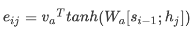Whererepresents the previous hidden layer output during the decoding phase. This formula has three calculation methods mentioned in the paper, which are as follows:

In the TensorFlow source code, the third calculation method is used.Thus, the core weights of Attention have been calculated. Next, let’s organize the entire process; the flow is shown in the diagram below:

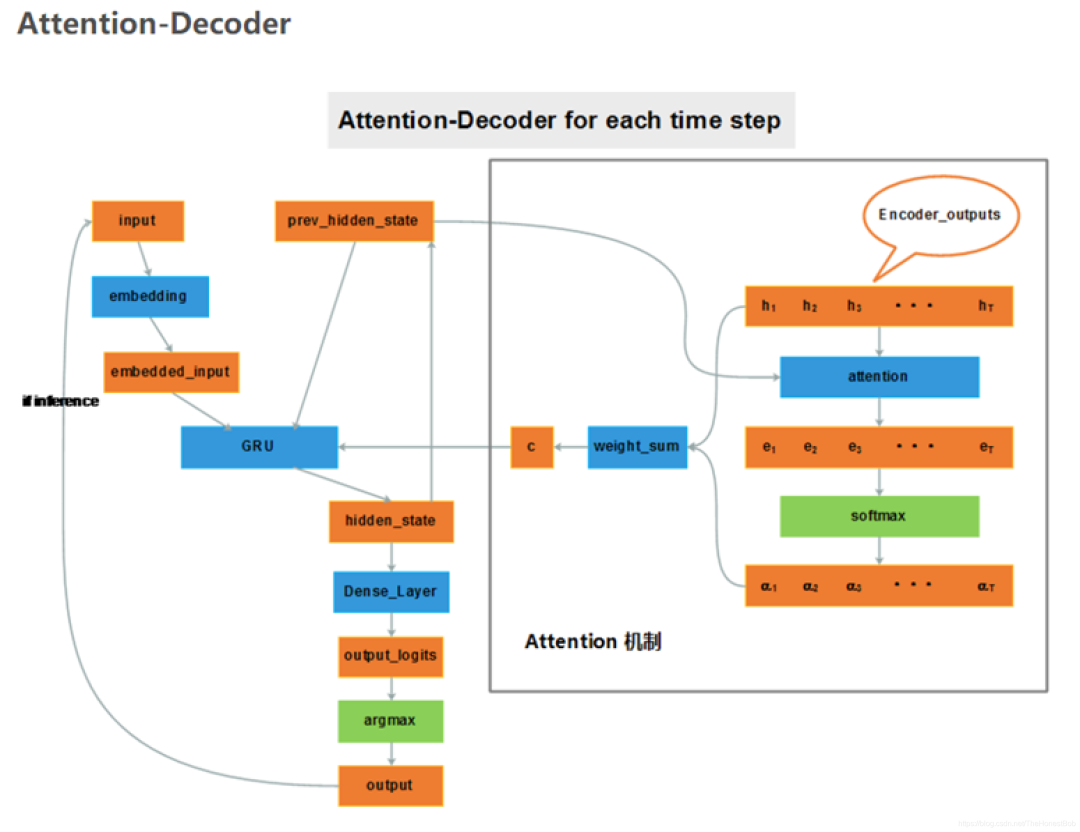
The gray box on the right shows the calculation process of the Attention mechanism. By tracing back through the formulas above, it should be clear. Note that the diagram only illustrates the decoding stage.We should not view the Attention mechanism as a standalone algorithm; it should be seen as a method. Once you grasp the essence of Attention, you can fully utilize your imagination to reasonably apply the Attention mechanism to achieve ideal results.Lastly, I would like to mention the difference between soft-attention and hard-attention. Soft-attention is the Attention mechanism we discussed above, which involves a weighted average of the outputs at each moment of decoding. It can directly obtain gradients;while hard-attention selects the output state of the encoding using a Monte Carlo sampling method. Those interested in this part can delve deeper.

3. My Understanding of the Attention Mechanism

Firstly, I know of two names for this mechanism: one is Attention, and the other is Alignment Model. I actually prefer to call it soft feature extraction. Because its essence is to select the feature value that has the greatest impact at each decoding moment. I believe that understanding the Attention mechanism in this way will greatly help us apply the Attention mechanism to other NLP tasks or other fields, such as the CV field. Of course, I currently do not know how the Attention mechanism is used in the CV field, but based on this understanding, I can speculate on application methods, such as distinguishing whether a picture is of a cat or a dog. After extracting features through our convolution, we can use the Attention mechanism to focus on the unique features of cats, capturing not only more valuable feature information but also reducing the impact of common features on the model’s classification performance, and even some noise from the image itself. We can even truncate parameters with weights below a threshold during inference, which can also help reduce inference time in certain scenarios. Of course, I hope to distinguish this from overfitting in deep learning; they are somewhat different. Secondly, through the process of solving the energy function, I personally believe that we can also adopt a similar approach when obtaining text similarity matching. Of course, these are merely personal speculations, and should not be considered as knowledge points; I just want to provide examples that can help beginners understand from another perspective, as the saying goes, “different strokes for different folks.”

3. Detailed Explanation of Transformer Principles

1. Overview

The inherent sequential nature of RNN causes the model to not be able to process samples in parallel. Of course, the so-called parallelism means that a sample cannot be processed simultaneously because there is a dependency between features. However, the effectiveness of the Attention mechanism is evident. So, is there a better method to solve the shortcomings while retaining the advantages? Thus, Transformer was born, followed closely by the birth of BERT. At this point, the NLP field has also ushered in the ImageNet era of the CV field (the era of transfer learning). The more powerful feature extraction capability provides strong semantic vector representations for complex NLP tasks, allowing NLP to further penetrate into everyone’s life. Of course, Attention is only part of the Transformer model structure, but it is also the most crucial part. I have previously translated the paper on Transformer; those who need it can refer to my translation of “Attention is All You Need.”

2. Principles of Transformer Structure

Since Transformer is an upgraded version of Attention, it must share similarities with Attention. Therefore, before introducing Transformer, it is necessary to explain the following three parameters: Q (Query): corresponds to the hidden layer output from the previous moment in the decoding end of the Attention mechanism. K (Key): corresponds to all hidden layer outputs in the encoding end of the Attention mechanism. V (Values): corresponds to the encoding vector C in the Attention mechanism. Allow me to complain a bit; most of the articles on Transformer written by experts online are not friendly at all for newcomers when explaining these three parameters. If these three parameters are not clearly explained, all the brilliant explanations that follow are in vain. With the above explanations, let’s revisit the explanations by the experts: it is equivalent to querying the corresponding V from K using the query vector Q. In other words, the model uses the hidden layer information Q from the previous moment to perform a weighted average (which is also Attention) with each hidden layer output K from the encoder, thus obtaining the current moment’s encoding vector V. I believe this explanation should clarify what QKV means. Of course, in the Transformer, it is self-attention. How is it self? In fact, we know that in the previous Attention mechanism, the QKV were all generated autoregressively (meaning that the current output depends on the previous output, referred to as AR). In self-attention, QKV are obtained by multiplying the input of the model with the corresponding matrix, so the paper states that self-attention is auto-encoding (AE). This is because in self-attention, there is no need to generate step by step as in RNN, which is also the reason why Transformer can be parallelized, which I have already mentioned earlier.

Overall Structure

First, here is the overall model structure from the paper:

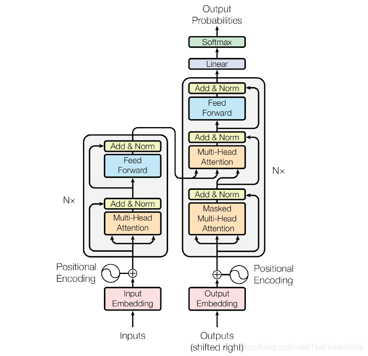
After all, it is a variant of Attention, and it cannot escape the end-to-end framework (this does not mean that the self-attention mechanism can only be used in an end-to-end framework; you can use it anywhere you need to extract features). In the paper, the left side shows six layers of Encoder, and the right side shows six layers of Decoder. The first layer in the Decoder is the Masked Multi-Head Attention layer. As for why it needs to be masked, it is mainly because our language model modeling is based on the word level. To obtain a sentence, we can only decode each word from left to right, masking future information. The reason we cannot directly predict a sentence is probably because the information between words is richer.

Input Embedding

Friends who are familiar with Transformer know that there is a positional information embedding here. The following diagram shows the positional encoding formula given in the paper:

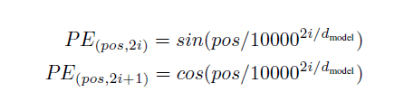
First, let’s explain each parameter:pos is the position of each token in the sequence, 2i and 2i+1 represent the even and odd dimensions of the vector for each token position, where all position indices start from 0,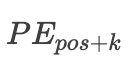is the dimension of the word vector, which is also the dimension of the positional encoding.The paper states that for a fixed K value,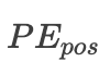can be represented as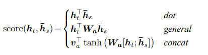linear function, what does this mean? It essentially means that the positional relationship between two tokens spaced K apart is linearly related. Next, we will derive how this linear relationship works. 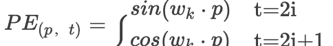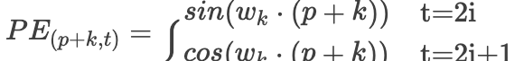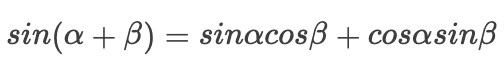For simplicity, let’s simplify the above formula:Then ourSince our trigonometric functions have the following transformations: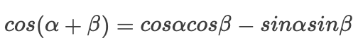Then we have:Since our k value is fixed, the terms related to k in the above expression are constants. Isn’t it a linear function concerningOf course, for self-encoding models like Transformer, the absence of positional information for tokens is crucial for sequence learning tasks, which also indicates that the quality of positional encoding methods directly affects the rationality of positional encoding information. Therefore, many improvements have been made to positional encoding, and I will delve into this in a separate blog post later.

Transformer Layer

This part I originally wrote some content, but later found that experts have written very well, and they have also included the feedforward neural network and residual connection I wanted to write about, so I will just link to the expert’s article. By deeply understanding RNN and Attention, it is no longer difficult to read articles, papers, and source code online, especially some papers related to improvements in the development of NLP.

Residual Connection

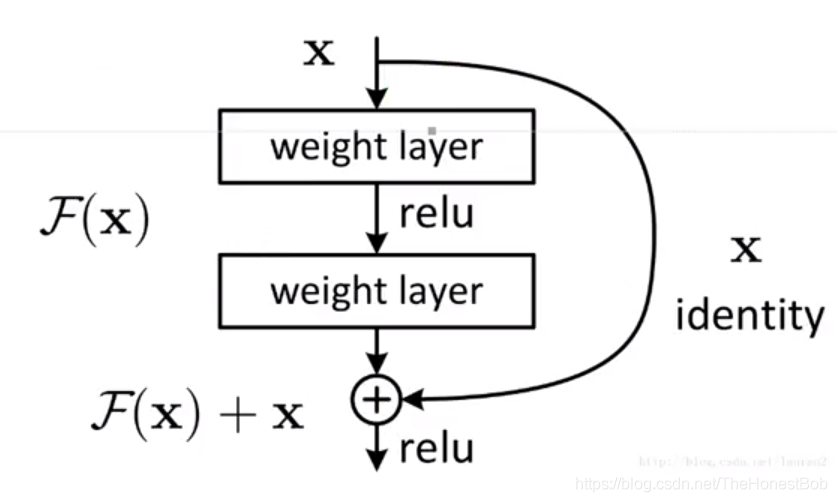
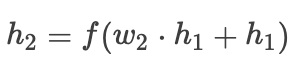
The structure of residual networks is quite simple, adding x back after skipping a few layers.It is said that residual networks effectively solve the gradient vanishing problem and the network degradation problem. But why is it effective? Let’s take a look at the formula to understand the effectiveness of residuals. First, I have drawn a simple computational graph, all of which are fully connected. To make the graph look clean, I simplified it a bit, and of course, it looks a bit ugly, haha. Let’s use this as an example to compute:

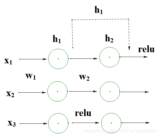
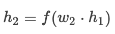
If we do not use residual connections, that is, omit the dashed part in the figure, the forward propagation is as follows:By the way, if you are not very clear about the principle of gradient descent, you can refer to my previous blog on the principles and calculations of the gradient descent algorithm.Then the gradient is: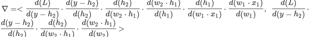whereis the activation function,is the hidden layer output,is the loss function,is the gradient.When we adopt residual connections, the forward propagation is as follows: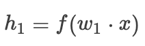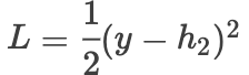Then the gradient is: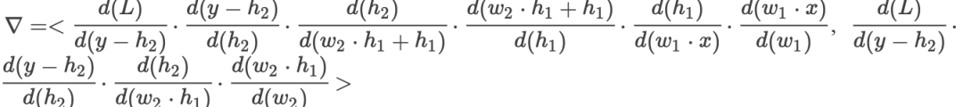where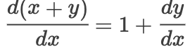By comparing, we find that in the first case, if the value of each partial derivative is very small, then in a very deep network structure, it will lead to very small gradient values, which means gradient vanishing, and the parameters will not be updated. However, after adding the residual, even in a very deep network, each partial derivative will add 1, thus allowing the error to propagate effectively and solving the gradient vanishing problem.As for the network degradation problem, it is essential to clarify that the concept of network degradation is due to the vast majority of parameter matrices stopping updates during backpropagation, which causes the network to lose its ability to continue learning. Because parameters do not update, it means that new samples do not contribute to network training, and the network has not learned the features of new samples.I have not yet delved deep into the issue of network degradation. I personally believe that it needs to be analyzed from the properties of the matrix rank and other characteristics that lead to parameter updates stopping.

3. Personal Understanding

In fact, for Transformer, the main improvements lie in parallelization and obtaining semantic information from long sequences. The reason it can be parallelized is that the three vectors QKV required for self-attention are obtained through three linear transformations of the input, instead of needing to complete all time steps as in traditional RNN. The ability to obtain longer semantic information lies in the fact that in self-attention, each Q can multiply with the original K to obtain the corresponding V, rather than the traditional attention where Q and K lose long-distance information due to the forward propagation in RNN. Of course, later Transformer-XL was proposed, and recently Google experts proposed a new kernel called Synthesizer to replace Transformer. Here I will post the paper link; I must admire the creativity of the experts. Carefully savoring these masterpieces and understanding them deeply will inspire us in many other ways, such as the positional encoding method in Transformer. Since deep learning now has powerful feature extraction capabilities, it is essential to consider how to incorporate more types of features into our data.

4. Detailed Explanation of BERT Principles

1. Overview

Actually, by now, BERT seems less mysterious than before. BERT utilizes the encoder of Transformer. If anyone needs it, they can refer to my previous BERT paper translation. BERT does not have much novelty in its model structure. The main reason it achieves good results is primarily due to the powerful feature extractor, Transformer, and secondly, it relies on two self-supervised language models. BERT marks the beginning of the ImageNet era in the NLP field, pre-training the network on a large corpus to initialize parameters, and then fine-tuning using a small amount of specialized domain data to achieve objective results. First, let’s look at the overall structure of BERT:

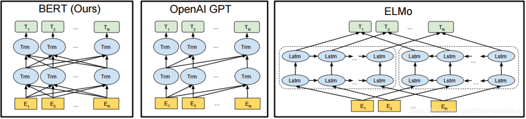
From the diagram, we can see that the overall structure of BERT is multiple stacked Transformer structures, where each column of Transformer performs the same operation, with the complete input of the sequence, and there is not much difference from Transformer.Next, we will mainly look at the language models used in BERT and how some specific tasks are completed, which may inspire us to have more solutions in algorithm development.

2. Language Models in BERT

MLM Language Model

In BERT, to train the input parameters, a self-supervised approach is adopted to pre-train on a large-scale corpus. For the word level, the MLM (Masked LM) is used, and the main process and method are as follows: 1. Randomly mask 15% of all tokens in the input sequence, using the [MASK] token, which must be included in the vocabulary. The training objective is to predict these tokens. 2. The paper also mentions that since the [MASK] token does not exist during prediction, to mitigate the mismatch between training and prediction, my understanding of this mismatch is that although only 15% of tokens are masked in a sequence, the percentage is not high, but the base number is significant. It is equivalent to the model learning some features of the [MASK] token during training, and 15% is quite a lot. So why did the author not mask fewer tokens? It is evident that the purpose of the mask operation is to train the self-supervised model. If too few tokens are masked, it would be meaningless. So what measures did the author take to alleviate this problem? The answer is to adopt the following strategies for the 15% of masked tokens: (1) With an 80% probability, use the [MASK] token (2) With a 10% probability, use a random token (3) With a 10% probability, do not replace the token. Why does this approach resolve the aforementioned issue? Under the condition of masking 15% of tokens, reducing the probability of the [MASK] token appearing by 20% means that for the remaining 20%, using random tokens would lead to incorrect learning because you are providing the network with incorrect samples. For example, if you want to predict the token ‘天’, but you randomly provide the token ‘地’, it creates a human error sample. Therefore, there is a 10% probability of using the original token, and the errors generated by random replacements are only 15%*10%=1.5%, which is not a significant issue for the model. It does not create much disturbance, just like how you use Python at work, but your knowledge of Java is incorrect; it does not affect you much since you do not use Java. Now you may ask, is there a difference between not replacing and not replacing from the start? The answer is yes because, for the model, you do not know whether the input is the real token or not, so the model can only predict based on the context, thereby achieving the training objective. It is like when an unreliable friend tells you that he found 100 yuan on the road; you do not know whether what he said is true or false, so you can only judge the credibility of his words based on other evidence.

NSP Language Model

For sentence-level tasks, BERT also provides an effective method (later papers have verified that the NSP task may not be so essential; this issue will not be discussed here), which is to predict whether the next sentence is true based on the previous sentence. Why propose this pre-training task? The main reason is that many tasks, such as question answering and reasoning, require learning the relationships between sentences, which cannot be accomplished by language models because language models learn within the sentence by predicting tokens. NSP is designed to capture dependencies between sentences, and the NSP task can be performed through self-supervised learning in a single corpus, where there is a 50% probability that the next sentence is true and a 50% probability that it is randomly selected from the corpus. Of course, the paper also mentions that using document-level corpora is far superior to unordered sentence corpora; this is very evident. Similar to the MLM language model, self-supervision is its greatest advantage.

Fine-tuning

BERT can be considered a semi-supervised process. After the self-supervised pre-training, we still need our specialized domain data to fine-tune the model parameters, thus better adapting it to our network. Next, I will briefly introduce the various tasks mentioned in the paper, first providing an overall task diagram.

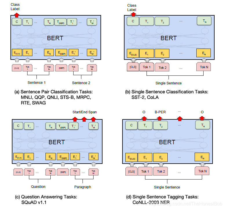
MNLI(Multi-Genre Natural Language Inference):Given a pair of sentences, the goal is to predict whether the second sentence is related to, irrelevant to, or contradicts the first sentence.QQP(Quora Question Pairs):Determine whether two questions have the same meaning.QNLI(Question Natural Language Inference):The sample is (question, sentence) to determine whether the sentence is the answer to the question in a text.STS-B(Semantic Textual Similarity Benchmark):Given a pair of sentences, use a rating of 1-5 to evaluate their semantic similarity.MRPC(Microsoft Research Paraphrase Corpus):The sentence pairs come from comments on the same news. Determine whether these two sentences are semantically the same.RTE(Recognizing Textual Entailment):This is a binary classification problem similar to MNLI, but the data volume is much smaller.SST-2(The Stanford Sentiment Treebank):This is a binary classification problem for single sentences, with sentences coming from people’s evaluations of a movie, determining the sentiment of the sentence.CoLA(The Corpus of Linguistic Acceptability):This is a binary classification problem for single sentences, determining whether an English sentence is grammatically acceptable.SQuAD(Stanford Question Answering Dataset):Given a question and a paragraph from Wikipedia that contains the answer, the task is to predict the position of the answer in the paragraph.CoNLL-2003 NERNamed Entity Recognition task, which should be familiar to everyone, predicting what label each character has.For the SQuAD task, the paper explains it in detail, and everyone can refer to my translated paper.In general, for tasks in (a) and (b), we obtain the final value of the CLS token.For tasks in (c), the main goal is to predict the start and end tokens’ positions, ensuring that the start token’s id is less than the end token’s id, where the start is the starting position of the answer in the paragraph, and the end is the ending position.For the NER task, we naturally obtain the values for each output since each token corresponds to a label.The BERT source code also provides a binary classification code example, which we can modify to train our tasks.

3. Personal Understanding

In fact, the most important inspiration that BERT gives me is self-supervision. Currently, deep learning is mostly supervised learning, which makes the data cost very high and thus restricts model training. Self-supervised learning can easily obtain data and complete basic model training when our task requirements are not high, effectively assisting in completing our main tasks. Recently, GPT-3 has also become popular, claiming to eliminate the need for fine-tuning, directly using the output features, with a total of 170 billion parameters. I was stunned. Personally, I feel that such a behemoth is not as good as XLNet, RoBERTa, ALBERT, XLNet, etc. There are also many articles online written by experts. My knowledge is limited, so I will just post the links. I spent some time writing this blog to get here. I work during the day and stay up late to write, so my head is a bit confused. I will write for now; I really can’t write anymore. I hope this helps everyone, and remember to give a thumbs up!

This article is authorized by the author AINLP and published on the public account platform. Contributions are welcome; AI and NLP are both acceptable.Due to formatting issues on the public account, some formulas may not display clearly. You can read the original text for clarity.Original link, click “Read Original” to go directly:

Repository address sharing:

Reply "code" in the backend of the Machine Learning Algorithms and Natural Language Processing public account to get access to 195 NAACL + 295 ACL 2019 papers with open-source code. The open-source address is as follows: https://github.com/yizhen20133868/NLP-Conferences-Code

Heavy news! The Yizhen Natural Language Processing - Pytorch group has been officially established! There are a lot of resources in the group; everyone is welcome to join and learn! 
Note: Please modify your remarks when adding as [School/Company + Name + Direction] For example — Harbin Institute of Technology + Zhang San + Dialogue System. 
The account owner, please avoid being a micro-business. Thank you!

Recommended reading:
Summary and thoughts on commonly used normalization methods: BN, LN, IN, GN
LSTM that everyone can understand
Comprehensive analysis of Python "partial function" usage