

Selected from | Lilian Weng’s blog
Author | Lilian Weng
Editor | Zhao Yang
This article is a review blog that explores and summarizes the commonly used large transformer efficiency optimization schemes.
Large Transformer models have become mainstream, creating SOTA results for various tasks. Indeed, these models are powerful, but they are very costly to train and use, with extremely high inference costs in terms of time and memory. In summary, the difficulties of using large Transformer models for inference include not only the increasing size of the models but also two significant factors:
-
High memory consumption: During inference, both model parameters and intermediate states need to be stored in memory. For example, the contents in the cache under the KV storage mechanism need to be stored in memory during decoding. For instance, with a batch size of 512 and a context length of 2048, the space required for the KV cache is 3TB, which is three times the model size; the inference cost of the attention mechanism is positively correlated with the input sequence length;
-
Low parallelism: The inference generation process is executed in an autoregressive manner, making the decoding process difficult to parallelize.
In this article, Lilian Weng, who leads application research at OpenAI, wrote a blog introducing several methods to improve transformer inference efficiency. Some are general network compression methods, while others apply to specific transformer architectures.
Lilian Weng is currently the head of application AI research at OpenAI, primarily engaged in research on machine learning, deep learning, etc. She graduated with a bachelor’s degree from the University of Hong Kong, a master’s degree from Peking University in Information Systems and Computer Science, and then pursued a PhD at Bruton University in India.

Model Overview
The following are generally regarded as the goals of model inference optimization:
-
Use fewer GPU devices and less GPU memory to reduce the memory footprint of the model;
-
Reduce the required FLOP to lower computational complexity;
-
Reduce inference latency and run faster.
Several methods can be used to lower the memory cost of the inference process and speed it up.
-
Apply various parallel mechanisms across multiple GPUs to achieve model scaling. Intelligent parallelization of model components and data makes it possible to run large models with trillions of parameters;
-
Unload temporarily unused data to the CPU and read it back when needed later. This is memory-friendly but can lead to higher latency;
-
Smart batching strategies; for example, EffectiveTransformer packs consecutive sequences together to eliminate padding in a single batch;
-
Neural network compression techniques, such as pruning, quantization, and distillation. Smaller models in terms of parameter count or bit width should require less memory and run faster;
-
Improvements specific to target model architectures. Many changes in architectures, especially changes in attention layers, help to improve the decoding speed of transformers.
This article focuses on network compression techniques and improvements to transformer models under specific architectures.
Quantization Strategies
There are two common methods to apply quantization strategies on deep neural networks:
-
Post-training quantization (PTQ): First, the model needs to be trained to convergence, and then its weight precision is reduced. Compared to the training process, quantization operations are often much less costly;
-
Quantization-aware training (QAT): Apply quantization during pre-training or further fine-tuning. QAT can achieve better performance but requires additional computational resources and representative training data.
It is worth noting that the theoretically optimal quantization strategies have an objective gap with actual performance on hardware kernels. Due to the lack of support for certain types of matrix multiplications (e.g., INT4 x FP16) in GPU kernels, not all methods below will accelerate the actual inference process.
Transformer Quantization Challenges
Many studies on quantizing Transformer models have the same observation: simply quantizing parameters to low precision (e.g., 8 bits) after training leads to significant performance degradation, mainly because the conventional activation function quantization strategies cannot cover the entire value range.
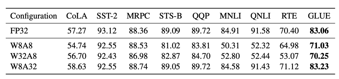
Figure 1. Quantizing model weights to 8 bits while using full precision for activation functions achieves better results (W8A32); when the activation function is quantized to 8 bits, the performance is worse than W8A32 regardless of whether weights are low precision (W8A8 and W32A8).
Bondarenko et al. observed in a small BERT model that due to strong outliers in the output tensor, the input and output of the FFN have very different value ranges. Therefore, quantizing the residuals of the FFN tensor one by one may lead to significant errors.
As the scale of model parameters continues to grow to the billions, high-magnitude outlier features begin to appear in all transformer layers, leading to poor performance of simple low-bit quantization. Dettmers et al. observed this phenomenon in OPT models with more than 6.7B parameters. Larger models also have more network layers with extreme outlier values, which greatly affect model performance. The scale of outlier activations in several dimensions can be about 100 times larger than most other values.
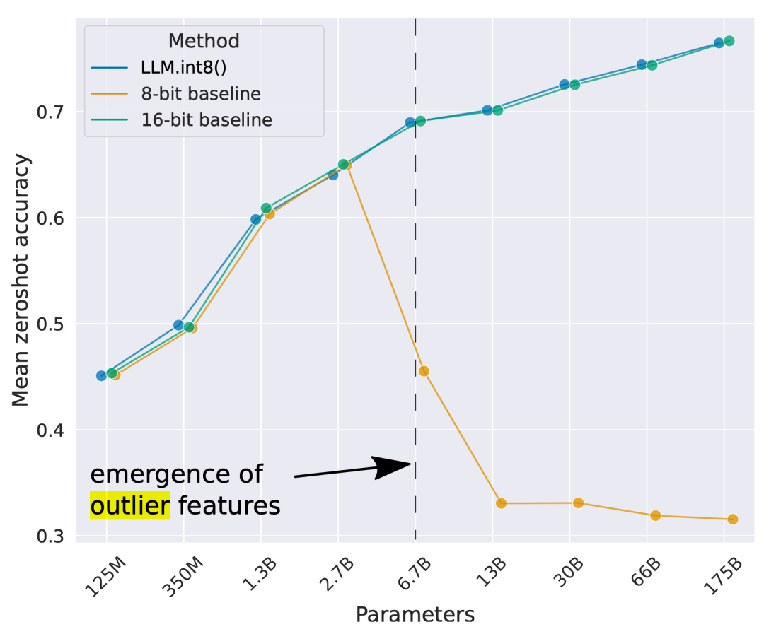
Figure 2. Average zero-shot accuracy of different scales of OPT models on four language tasks (WinoGrande, HellaSwag, PIQA, LAMBADA).
Mixed Precision Quantization
The most straightforward way to solve the above quantization challenges is to quantize weights and activation functions with different precisions.
GOBO model is one of the first models to apply post-training quantization to transformers (i.e., small BERT model). GOBO assumes that the model weights of each layer follow a Gaussian distribution, thus detecting outliers by tracking the mean and standard deviation of each layer. Outlier features maintain their original form, while other values are grouped into multiple bins, and only the corresponding weight indices and centroid values are stored.
Based on the observation that only certain activation layers in BERT (e.g., the residual connections after FFN) lead to significant performance degradation, Bondarenko et al. adopted mixed precision quantization by using 16-bit quantization on problematic activation functions and 8-bit on others.
Mixed precision quantization in LLM.int8() is achieved through two mixed precision decompositions:
-
Since matrix multiplication involves independent inner products between a set of row and column vectors, each inner product can be quantized independently. Each row and column are scaled by the maximum value and then quantized to INT8;
-
Outlier activation features (e.g., those larger than 20 times other dimensions) remain in FP16, but they only account for a tiny portion of the total weights, although outliers need to be empirically identified.
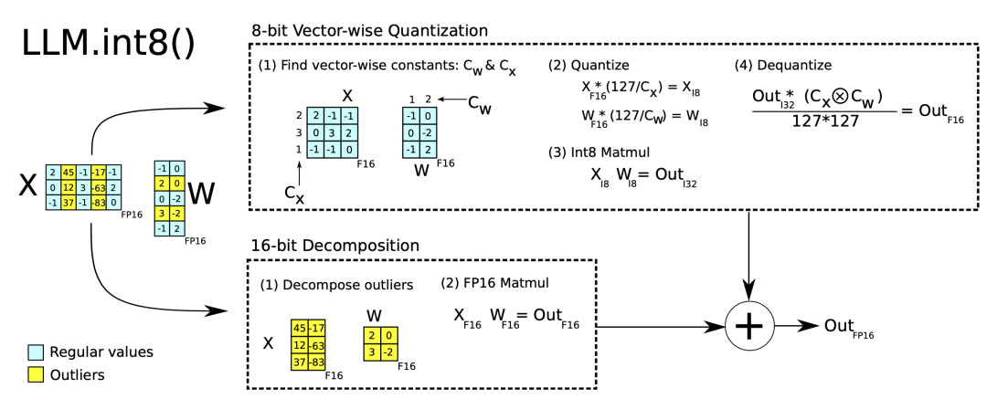
Figure 3. Two mixed precision decomposition methods in LLM.int8().
Fine-Grained Quantization
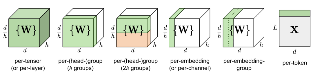
Figure 4. Comparison of different granularities of quantization. d is model size / hidden space dimension, h is the number of heads in a MHSA (multi-head self-attention) component.
Simply quantizing the entire weight matrix in a layer (tensor-wise or layer-wise quantization) is the easiest to implement, but the quantization granularity is often unsatisfactory.
Q-BERT applies grouped quantization to fine-tuned BERT models, treating each matrix W of each head in MHSA (multi-head self-attention) as a group, and then applying mixed precision quantization based on the Hessian matrix.
The design motivation for per-embedding group (PEG) activation function quantization is the observation that outliers only appear in a few dimensions. Quantizing each embedding layer is very costly; in contrast, PEG quantization divides the activation tensor along the embedding dimension into several uniformly sized groups, where elements within the same group share quantization parameters. To ensure that all outliers are grouped together, PEG applies an embedding dimension arrangement algorithm based on value ranges, where dimensions are sorted by their value ranges.
ZeroQuant, like Q-BERT, applies grouped quantization to weights and also uses a token-wise quantization strategy for activation functions. To avoid the costly quantization and dequantization computations, ZeroQuant builds unique kernels to fuse quantization operations with their preceding operators.
Using Second-Order Information for Quantization
Q-BERT developed Hessian Aware Quantization (HAWQ) for mixed precision quantization. The motivation is that parameters with higher Hessian spectra are more sensitive to quantization, thus requiring higher precision. This method is essentially a way to identify outliers.
From another perspective, the quantization problem is an optimization problem. Given a weight matrix W and an input matrix X, the goal is to find a quantized weight matrix W^ that minimizes the following MSE loss:
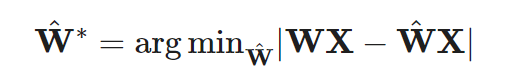
GPTQ views the weight matrix W as a collection of row vectors w and quantizes each row independently. GPTQ uses a greedy strategy to select weights that need to be quantized and iteratively quantizes them to minimize quantization error. Updating the selected weights generates a closed-form solution in the form of a Hessian matrix. GPTQ can reduce the weight bit width in OPT-175B to 3 or 4 bits without significant performance loss, but it is only applicable to model weights, not activation functions.
Outlier Smoothing
It is well known that activation functions in Transformer models are more difficult to quantize than weights. SmoothQuant proposes an intelligent solution that smooths outlier features from the activation functions to the weights through mathematically equivalent transformations, and then quantizes both weights and activation functions (W8A8). As a result, SmoothQuant has better hardware efficiency than mixed precision quantization.
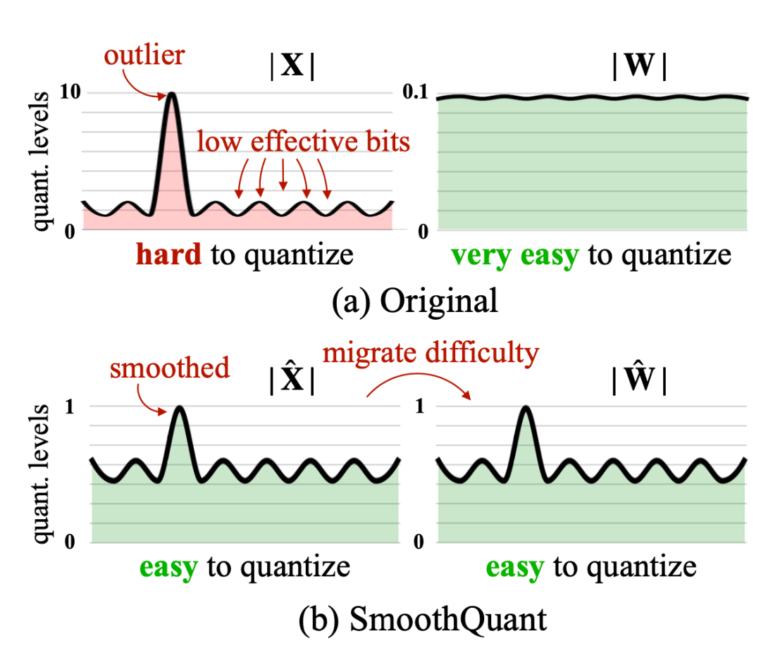
Figure 5. SmoothQuant transfers scale variance from activation functions to offline weights to reduce the difficulty of quantizing activation functions. The resulting new weight and activation matrices are both easy to quantize.
Based on the per-channel smoothing factor s, SmoothQuant scales weights according to the following formula:
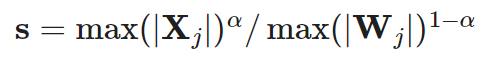
According to the smoothing factor it can be easily fused into the parameters of the previous layer in an offline state. The hyperparameter α controls the degree of transfer from activation functions to weights. The study found that α=0.5 is the optimal value for many LLMs in the experiments. For models with larger activation outliers, α can be increased.
Quantization-Aware Training (QAT)
Quantization-aware training integrates quantization operations into the pre-training or fine-tuning process. This approach directly learns the model weights in low-bit representations, achieving better performance at the cost of additional training time and computation.
The most direct method is to fine-tune the model after quantizing on the same or representative training dataset as the pre-training dataset. The training objective can be the same as the pre-training objective (e.g., NLL/MLM in general language model training) or specific to downstream tasks (e.g., cross-entropy for classification).
Another method is to treat the full-precision model as a teacher model and the low-precision model as a student model, then optimize the low-precision model using distillation loss. Distillation usually does not require using the original dataset.
Pruning
Network pruning reduces model size by trimming unimportant model weights or connections while retaining model capacity. Pruning may or may not require retraining. Pruning can be unstructured or structured.
-
Unstructured pruning allows the removal of any weights or connections, so it does not preserve the original network architecture. Unstructured pruning is often more demanding on hardware and does not accelerate actual inference;
-
Structured pruning does not change the sparsity of the weight matrix itself and may need to follow certain pattern constraints to utilize content supported by hardware kernels. This article focuses on structured pruning that can achieve high sparsity in transformer models.
The typical workflow for building a pruned network includes three steps:
1. Train a dense neural network to convergence;
2. Prune the network to remove unnecessary structures;
3. (Optional) Retrain the network to maintain the previous training performance with the new weights.
The inspiration for discovering sparse structures in dense models through pruning while still maintaining similar performance comes from the lottery hypothesis: a randomly initialized dense feedforward network contains a pool of subnetworks, only one subset (the sparse network) is the winning ticket, which can achieve optimal performance when trained independently.
How to Prune
Magnitude pruning is the simplest yet highly effective pruning method – only pruning those weights with the smallest absolute values. In fact, some studies have found that simple magnitude pruning methods can achieve comparable or even better results than complex pruning methods such as variational dropout and l_0 regularization. Magnitude pruning is easy to apply to large models and achieves relatively consistent performance over a considerable range of hyperparameters.
Zhu & Gupta found that large sparse models can outperform small but dense models. They proposed the Gradual Magnitude Pruning (GMP) algorithm, which gradually increases the sparsity of the network during training. In each training step, weights with the smallest absolute values are masked to zero to achieve the desired sparsity, and masked weights do not receive gradient updates during backpropagation. The required sparsity increases as the training steps progress. The GMP process is sensitive to learning rate scheduling; the learning rate should be higher than that used in dense network training but not too high to prevent divergence.
Iterative pruning repeatedly executes step 2 (pruning) and step 3 (retraining) of the above three steps, pruning only a small portion of weights each time, and retraining the model in each iteration. This process is continuously repeated until the desired level of sparsity is achieved.
How to Retrain
Retraining can be achieved through simple fine-tuning using the same pre-training data or other task-specific datasets.
The Lottery Ticket Hypothesis proposes a weight rewinding retraining method: after pruning, the unpruned weights are reinitialized to their original values from the early stages of training, then retrained with the same learning rate schedule.
Learning rate rewinding only resets the learning rate to its earlier value while keeping the unpruned weights unchanged since the last training phase ended. Researchers observed that (1) retraining with weight rewinding outperformed retraining through fine-tuning across networks and datasets, and (2) in all test scenarios, learning rate rewinding performed equally well or even better than weight rewinding.
Sparsification
Sparsification is an effective method to expand model capacity while maintaining model inference computational efficiency. This article considers two types of transformer sparsity:
-
Sparsified fully connected layers, including self-attention layers and FFN layers;
-
Sparse model architectures, such as the merging operations of MoE components.
N:M Sparsification Achieved through Pruning
N:M sparsification is a structured sparsification pattern that is optimized for modern GPU hardware, where N out of every M consecutive elements are zero. For example, the NVIDIA A100 GPU’s sparse tensor cores support 2:4 sparsity to accelerate inference.
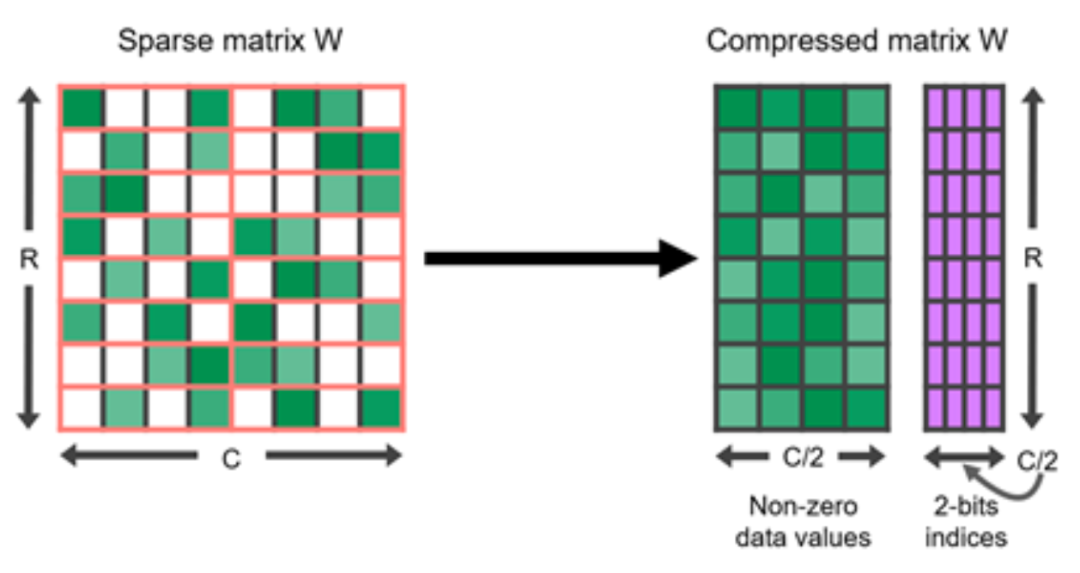
Figure 6. 2:4 structured sparse matrix and its compressed representation.
To make the sparsification of dense neural networks follow the N:M structured sparsification pattern, NVIDIA recommends a three-step operation to train the pruned network: train –> prune to meet 2:4 sparsity –> retrain.
(1) Rearranging the columns of a matrix can provide more possibilities during the pruning process to maintain the number of parameters or meet special constraints such as N:M sparsity. As long as the axes of the two matrices are arranged in the same order, the result of matrix multiplication remains unchanged. For example, (1) in the self-attention module, if the axis 1 of the query embedding matrix Q and the axis 0 of the key embedding matrix K^⊤ are arranged in the same order, the result of QK^⊤ matrix multiplication remains unchanged.
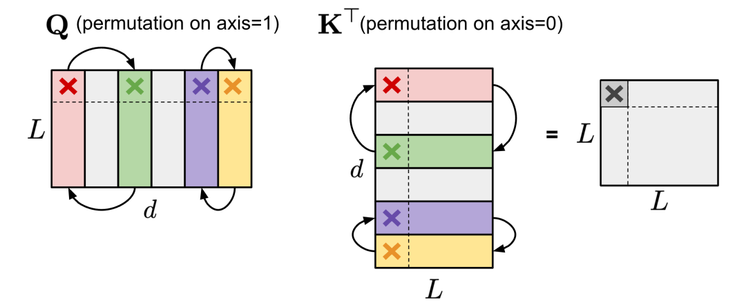
Figure 7. Same arrangement on Q (axis 1) and K^⊤ (axis 0) results in unchanged outcomes in the self-attention module.
(2) Within an FFN layer containing two MLP layers and a ReLU non-linear layer, the first linear weight matrix W_1 can be arranged along axis 1, and the second linear weight matrix W_2 can be arranged along axis 0 in the same order.
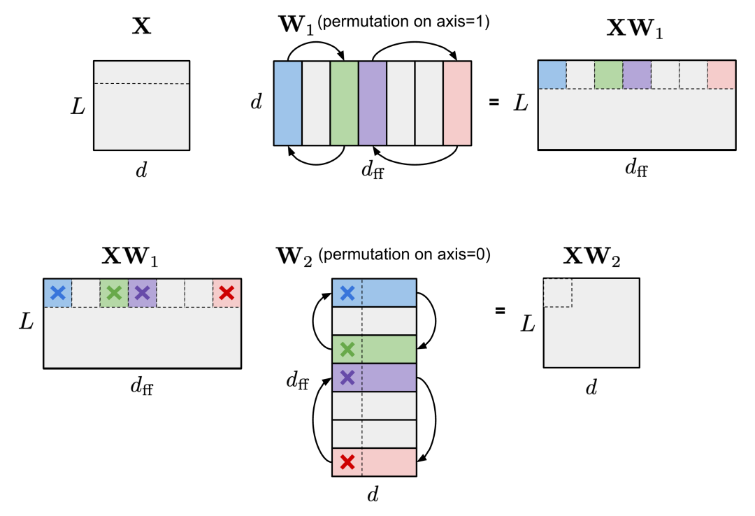
Figure 8. The same arrangement on W_1 (axis 1) and W_2 (axis 0) keeps the output of the FFN layer unchanged. For simplicity, the bias terms are omitted in the illustration but should also be applied with the same arrangement.
To promote N:M structured sparsification, the columns of one matrix need to be split into multiple slides (also known as stripes) of M columns, making it easy to observe the column order within each stripe and the order of stripes that impose restrictions on N:M sparsification.
Pool and Yu proposed an iterative greedy algorithm to find the optimal arrangement to maximize the weight magnitude of N:M sparsification. All channel pairs are speculatively swapped, and only the swaps that yield the largest magnitude increase are adopted, generating a new arrangement and ending a single iteration. Greedy algorithms may only find local minima, so they introduced two techniques to escape local minima:
1. Bounded regression: In practice, the maximum number of swaps between two random channels is fixed. Each search only allows one channel to be swapped to keep the search space wide and shallow;
2. Narrow and deep search: Select multiple stripes and optimize them simultaneously.
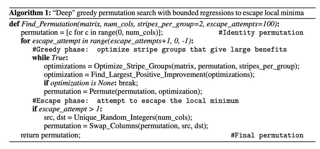
Figure 9. Greedy algorithm iteratively seeks the optimal arrangement for N:M sparsification.
Compared to pruning the network in default channel order, better performance can be achieved if the network is permuted before pruning.
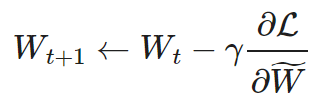
To train models with N:M sparsification from scratch, Zhou & Ma extended the STE commonly used in model quantization for magnitude pruning and sparse parameter updates.
STE computes the gradients of the dense parameters of the pruned network and applies it as an approximation to the dense network W:
STE’s extended version, SR-STE (Sparse Refinement STE), updates the dense weights W as follows:
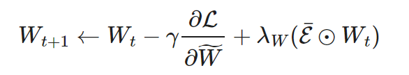
where is the mask matrix, ⊙ is element-wise multiplication. SR-STE prevents drastic changes in the binary mask by (1) constraining the pruning of weights in
 and (2) maintaining the unpruned weights in
 to prevent drastic changes in the binary mask.
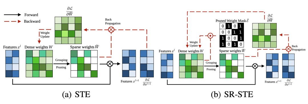
Figure 10. Comparison of STE and SR-STE. The comparison of ⊙ is element-wise product; ⊗ is matrix multiplication.
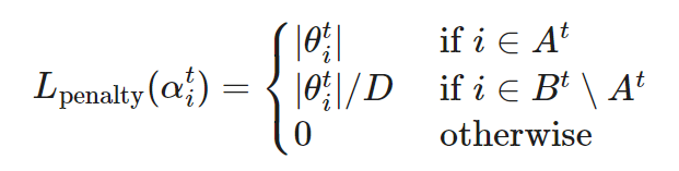
Unlike STE or SR-STE, the Top-KAST method can maintain constant sparsity throughout the entire training process of forward and backward propagation without requiring a forward pass with dense parameters or gradients.
During training at step t, the Top-KAST process is as follows:
Sparse forward pass: Select a subset of parameters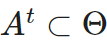 that includes the top K parameters per layer arranged by size, limited to the top D proportion of weights. If the parameterization α^t at time t is not in A^t (active weights), it is parameterized to zero.
where TopK (θ,x) selects the top x weights from θ after sorting by size.
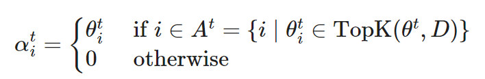
Sparse backward pass: Then apply gradients to a larger subset of parameters , where B contains (D+M), and A⊂B. Expanding the proportion of weights to be updated allows for more effective exploration of different pruning masks, thus increasing the chances of aligning the top D% of active weights.
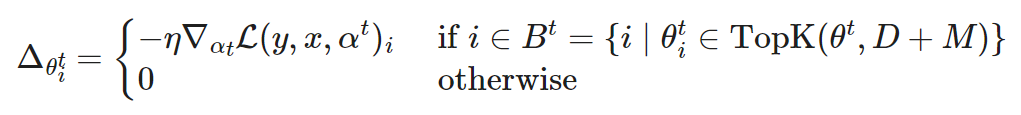
Training is divided into two stages, where additional coordinates in B∖A control the amount of exploration introduced. The exploration amount gradually decreases during training, and the final mask stabilizes.
Figure 11. The pruning mask of Top-KAST stabilizes over time.
To prevent the Matthew effect, Top-KAST penalizes active weights through L2 regularization loss to encourage more new exploration. During updates, parameters in B∖A are penalized more than those in A to stabilize the mask.
Sparse Transformer
Sparse Transformers sparsify the self-attention and FFN layers in the Transformer architecture, achieving a 37-fold speedup in single-sample inference.
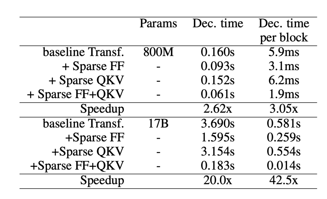
Figure 12. When applied to different network layers, the speed of the Transformer model decoding a single token (non-batch inference).
Sparse FFN layers: Each FFN layer consists of 2 MLPs and an intermediate ReLU. Since ReLU introduces many zero values, this method designs a fixed structure on the activation functions to enforce that only one non-zero value exists in a block containing N elements. The sparsity pattern is dynamic, differing for each token.
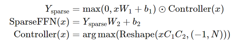
Each activation function result in Y_(sparse) corresponds to a column in W_1 and a row in W_2. The controller is a low-rank bottleneck fully connected layer, where ,
, use argmax for inference during training to select which columns should be non-zero. Gumbel-softmax techniques are also employed. Since the controller can compute its output before loading the FFN weight matrix, it can determine which columns will be zeroed out, thereby avoiding loading them into memory for faster inference.
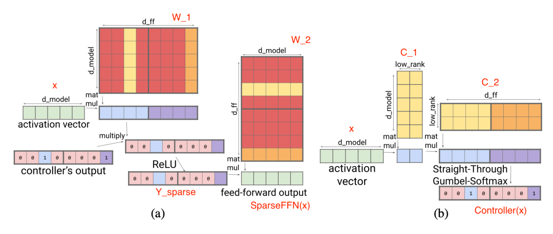
Figure 13. (a) Sparse FFN layer; the red columns are not loaded into memory for faster inference. (b) The controller of sparse FFN with 1:4 sparsity.
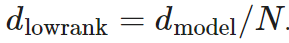
Sparse attention layers: In the attention layer, the dimension d_(model) is divided into S modules, each of size M=d_(model)/S. To ensure that each subdivision can access any part of the embedding, the Scaling Transformer introduces a multiplication layer (i.e., an element-wise multiplication layer that multiplies inputs from multiple neural network layers), which can represent any permutation but contains fewer parameters than a fully connected layer.
Given the input vector 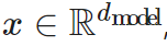 , the output of the multiplication layer is
  :
:
The output of the multiplication layer is a tensor of size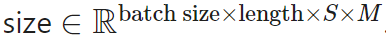 . It is then processed by a 2D convolution layer, where length and S are treated as the height and width of the image. Such a convolution layer further reduces the number of parameters and computation time in the attention layer.
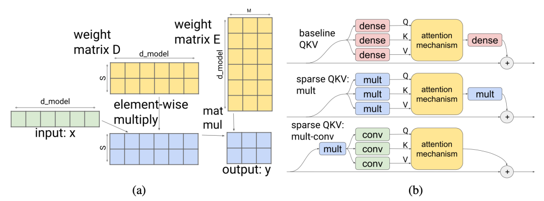
Figure 14. (a) Introducing a multiplication layer to allow partitions to access any part of the embedding. (b) The combination of multiplication fully connected layer and 2D convolution layer reduces the number of parameters and computation time in the attention layer.
To better handle long sequence data, the Scaling Transformer is further equipped with LSH (Locality Sensitive Hashing) attention and FFN block loops from Reformer, resulting in the Terraformer model.
Mixture of Experts (MoE)
The mixture of experts (MoE) models is a collection of expert networks, where only a subset of the network is activated for each sample to obtain prediction results. This idea originated in the 1990s and is closely related to ensemble methods. For detailed information on how to integrate MoE modules into Transformers, please refer to the previous posts by the author of this article on large model training techniques and the papers by Fedus et al. on MoE.
Using the MoE architecture, only a portion of the parameters are used during decoding, thus saving inference costs. The capacity of each expert can be adjusted through the hyperparameter capacity factor C, where the expert capacity is defined as:
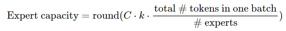
Each token needs to select the top k experts. A larger C expands expert capacity and improves performance, but this incurs higher computational costs. When C>1, a relaxation capacity needs to be increased; when C<1, the routing network needs to ignore some tokens.
Routing Strategy Improvements
The MoE layer has a routing network that assigns a subset of experts to each input token. The routing strategy in native MoE models routes each token to the preferred experts in the order they appear. If the routed expert has no extra space, the token is marked as overflowed and skipped.
V-MoE adds MoE layers to ViT (Vision Transformer). It matches the performance of previous SOTA models while requiring only half the inference computation. V-MoE can scale to fifteen million parameters. Researchers have experimented with k=2, requiring 32 bits per expert, with an MoE layer placed between every two experts.
Since each expert has limited capacity, if some important and informative tokens appear too late in the predefined sequence order (e.g., word order in sentences or patch order in images), they may have to be discarded. To avoid this flaw in the native routing scheme, V-MoE adopts BPR (Batch Priority Routing) to first assign experts to tokens with high priority scores. BPR calculates the priority score of each token before expert assignment (the maximum or sum of the scores of the top k routers) and rearranges the order of tokens accordingly. This ensures that core tokens can prioritize the use of the buffer of expert capacity.
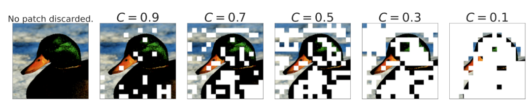
Figure 15. The way of discarding image patches when C<1 based on priority scores.
When C≤0.5, BPR performs better than ordinary routing, at which point the model begins to discard a large number of tokens. This allows the model to compete with dense networks even at very low capacities.
In researching how to explain the relationship between image categories and experts, researchers observed that earlier MoE layers are more general, while later MoE layers can specialize in certain types of images.
Task-level MoE takes task information into account and processes routing tokens from a task-level perspective. Researchers grouped translation tasks based on target languages or language pairs as an example of MNMT (Multilingual Neural Machine Translation).
Token-level routing is dynamic, and routing decisions for each token are mutually exclusive. Therefore, during inference, the server needs to preload all experts. In contrast, task-level routing is static, even fixed for tasks, so an inference server for a task only needs to preload k experts (assuming top-k routing exists). According to researchers’ experiments, task-level MoE can achieve performance gains similar to token-level MoE compared to dense model baselines, with peak throughput increased by 2.6 times and decoder size reduced by 1.6%.
Task-level MoE essentially classifies task distributions based on predefined heuristic methods, incorporating such human knowledge into routers. When such heuristics are absent, task-level MoE becomes difficult to use.
PR MoE allows each token to pass through a fixed MLP and a selected expert. Since later MoEs are more valuable, PR MoE designs more exits in the later layers. The DeepSpeed library implements flexible multi-expert and multi-data parallelism to support training PR MoE with different numbers of experts.
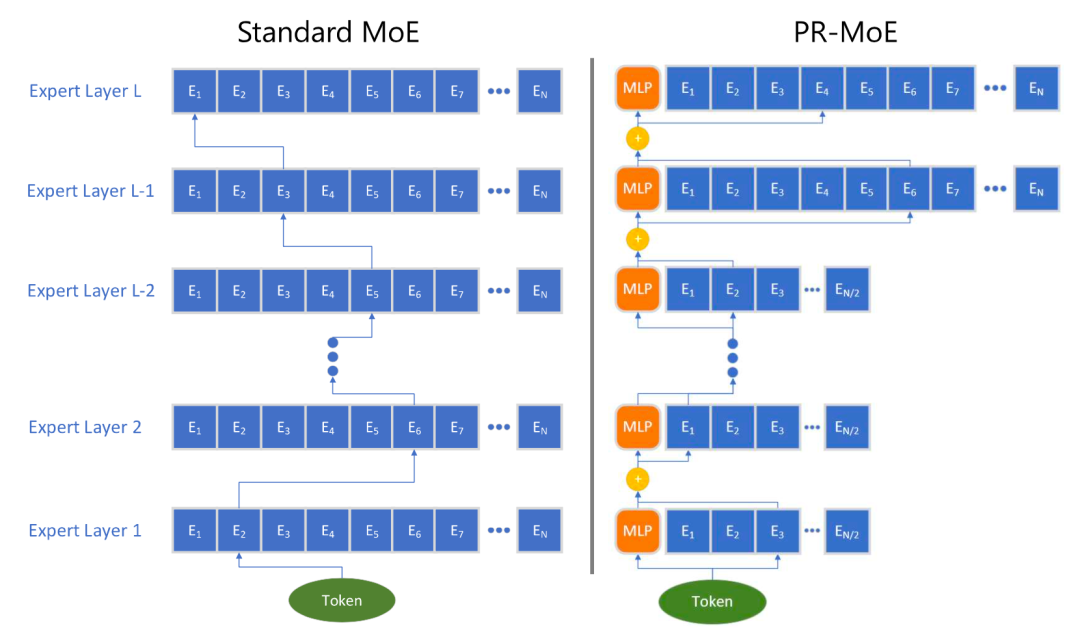
Figure 16. Comparison of PR MoE architecture with standard MoE.
Kernel Improvements
Expert networks can be hosted on different devices. However, as the number of GPUs increases, the number of experts on each GPU decreases, making communication costs between experts more expensive. The multi-to-multi communication between experts across multiple GPUs relies on the NCCL’s P2P API, which cannot occupy all the bandwidth of high-speed links, as the more nodes used, the smaller each chunk. Existing multi-to-multi algorithms perform poorly on large-scale problems, and the workload of a single GPU cannot be increased. To address this, several kernel improvements have been made to achieve more efficient MoE computations, such as making multi-to-multi communication cheaper/faster.
The DeepSpeed library and TUTEL implement a tree-based hierarchical multi-to-multi algorithm, which processes multi-to-multi communication within nodes and then implements multi-to-multi communication between nodes. This algorithm reduces the communication hops from O(G) to 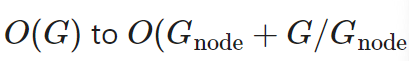 , where G is the total number of GPU nodes and G_(node) is the number of GPU kernels per node. Although the communication volume doubles in such implementations, it can better scale the batch size due to the latency of 1×1 convolution layers when the batch size is small.
DynaMoE uses dynamic recompilation to adapt computational resources to the dynamic workload between experts. The recompilation mechanism requires compiling the computation graph from scratch and reallocating resources only when needed. It fine-tunes the number of samples assigned to each expert and dynamically adjusts its capacity factor C to reduce runtime memory and computation requirements. This approach is based on observations of the allocation relationships between experts and samples in the early stages of training, introducing sample allocation caches after model convergence, and then using recompilation algorithms to eliminate dependencies between gating networks and experts.
Architecture Optimization
The paper “Efficient Transformers: A Survey” reviews a series of new Transformer architectures and suggests several improvements for enhancing computational and memory efficiency. Additionally, readers can refer to the article “The Transformer Family” for an in-depth understanding of various types of Transformer improvements.
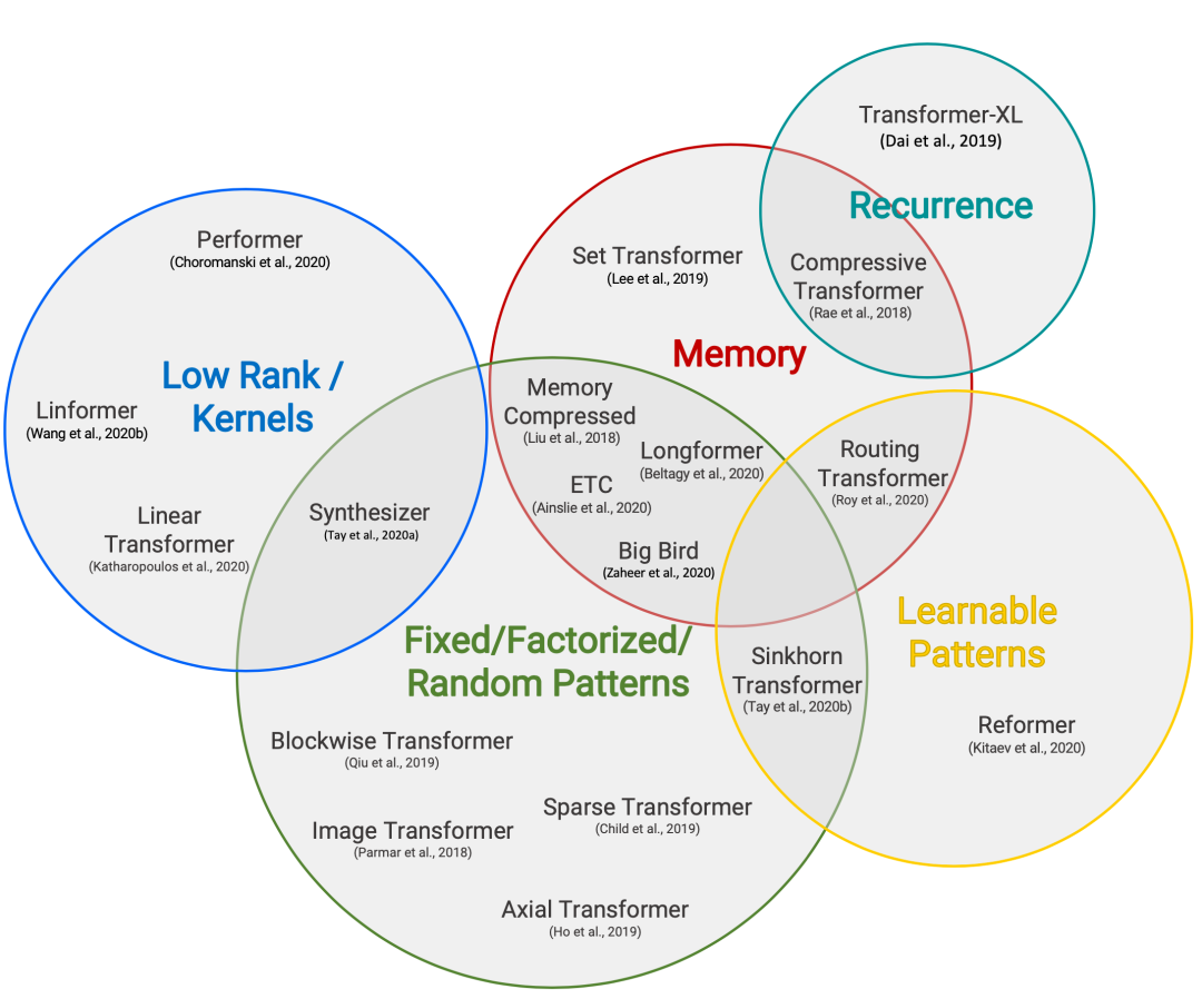
Figure 17. Classification of efficient transformer models
The secondary time complexity and memory complexity issues of the self-attention mechanism are the main bottlenecks in improving transformer decoding efficiency, thus all efficient transformer models apply some form of sparsification measures to the originally dense attention layers.
1. Fixed patterns: Use predefined fixed patterns to limit the receptive field of the attention matrix:
-
The input sequence can be divided into fixed blocks;
-
Image transformers use local attention;
-
Sparse transformers use cross-line attention patterns;
-
Longformer uses dilated attention windows;
-
Strided convolutions can be used to compress attention to reduce sequence length.
2. Combined patterns: Sort/cluster input tokens for a more optimized global view of the sequence while maintaining the efficiency advantages of fixed patterns
-
Sparse transformers combine strided and local attention;
-
Given high-dimensional input tensors, axial transformers do not flatten the input before using attention mechanisms but use multiple attention mechanisms, with one attention corresponding to one axis of the input tensor;
-
The Big Bird model designs several key components, namely (1) global tokens, (2) random attention (query vectors randomly bind to key vectors), and (3) fixed patterns (local sliding windows).
3. Learnable patterns: Learn to determine the best attention patterns:
-
Reformer uses locality-sensitive hashing to cluster tokens;
-
Routing transformers cluster tokens using k-means;
-
Sinkhorn sorting networks learn sorting algorithms for blocks of input sequences.
4. Recursive: Connect multiple blocks/segments recursively:
-
Transformer-XL reuses hidden states between segments to obtain longer context;
-
Universal transformers combine self-attention with the recurrent mechanism in RNNs;
-
Compressive transformers are extensions of Transformer-XL with additional memory, with n_m memory slots and n_(cm) compressed memory slots. Whenever a new input segment is fed into the model, the oldest activations in the main memory are transferred to the compressed memory.
5. Side Memory: Use Side Memory modules that can access multiple tokens at once
-
Set transformers design new attention mechanisms inspired by inductive point methods;
-
ETC (Extended Transformer Construction) is a variant of Sparse Transformer with a new global-local attention mechanism;
-
Longformer is also a variant of Sparse Transformer, using dilated sliding windows. As the model network deepens, the receptive field gradually increases.
6. Memory savings: Change the architecture to use less memory:
-
Linformer projects the dimension of key and value representatives to a low-dimensional representation (N→k), thus reducing memory complexity from N×N to N×k;
-
Shazeer et al. proposed multi-query attention, sharing keys and values among different attention heads, significantly reducing the size and memory cost of these tensors.
7. Using kernels: Using kernels can simplify the mathematical formulation of self-attention mechanisms. It is important to note that here, the kernel refers to the kernel in kernel methods, not GPU operators.
8. Adaptive attention: Let the model learn the optimal attention breadth or determine when to exit early for each token:
-
Adaptive attention breadth trains the model to learn the optimal attention breadth for each token and each attention head through a soft mask mechanism between tokens and other keys;
-
Universal transformers combine recurrent mechanisms and use ACT (Adaptive Computation Time) to dynamically decide how many times to loop;
-
Deep adaptive transformers and CALM use some confidence metrics to learn when to exit early at each layer of computation for each token, thus finding a balance between performance and efficiency.
Original link: https://lilianweng.github.io/posts/2023-01-10-inference-optimization/

Scan the QR code to add the assistant on WeChat
About Us