

1. Review DNN Training Word Vectors
Last time we discussed how to train word vectors using the DNN model. This time, we will explain how to train word vectors using word2vec.
Let’s review the DNN model for training word vectors that we discussed earlier:
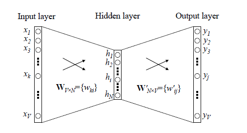
In the DNN model, we use the CBOW or Skip-gram mode combined with stochastic gradient descent. This means we only train on a few words from the training samples each time, and after each training, we perform backpropagation to update the weights W and W’ in the neural network.
We found that the DNN model still has two drawbacks:
First, we only use a few words for training each time, but during the gradient calculation, we have to compute the entire parameter matrix, which is inefficient.
The more important drawback is that when using softmax in the output layer, we need to calculate the probability for each position in the output layer. The softmax function is shown in the figure below:
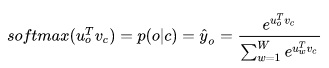
Here, u_0 is the parameter vector of a neuron in W’, and v_c corresponds to the vector obtained by multiplying the training sample with the hidden layer parameter W and then activating it. We can see that to get the probability for each position in the output layer, we need to compute the scores for all words, which can be resource-intensive if the vocabulary is large.
2. Word2vec
2.1 Overview
To address the drawbacks of DNN model training word vectors, in 2013, Google open-sourced a tool for calculating word vectors called word2vec, which attracted attention from both industry and academia. Word2vec uses two techniques, Hierarchical Softmax and Negative Sampling, to improve the performance of training word vectors. Due to space constraints, this time we will only explain the CBOW model optimized based on Hierarchical Softmax.
2.2 Huffman Tree
Before introducing the network structure of word2vec, we need to briefly review the Huffman tree. Given nodes with different weights w, we treat them as n trees in a forest. We first select the two nodes with the smallest weights w_i,w_j and merge them to form a new tree. The original w_i,w_j become the left and right subtrees of this new tree. The weight of the new tree is the sum of the weights of w_i and w_j, and we then treat the new tree as a new tree, deleting the original w_i,w_j trees, and repeat the process until all trees are merged. For example, if we have (a,b,c,d,e,f) with weights (16,4,8,6,20,3), we define the left branch as 0 and the right branch as 1.
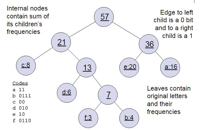
All words are leaf nodes, and the advantage of the Huffman tree is that words with larger weights (i.e., more frequent words) will be located at shallower leaf nodes, obtaining shorter codes. This way, more frequent words can be discovered with lower costs.
2.3 Hierarchical Softmax Network Structure
Word2vec has two optimized acceleration models: one based on Hierarchical Softmax optimization and the other based on Negative Sampling optimization. This time, we will only explain the model optimized based on Hierarchical Softmax. The following diagram shows the Word2vec model optimized using Hierarchical Softmax with the training mode selected as CBOW:
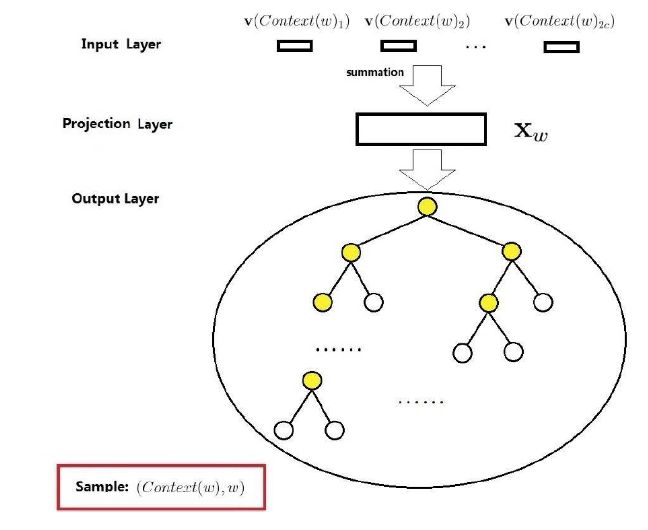
The network structure consists of three layers: the input layer, the projection layer (which is the original hidden layer), and the output layer. Assuming there exists a sample (Context(w),w), where Context(w) consists of w and c words before and after, it serves as the input sample train_X, and w serves as the output value train_y.
1)Input Layer:
Consists of 2c word vectors v(Context(w)_1),v(Context(w)_2),……,v(Context(w)_2c) that are all of the same length.
2)Projection Layer:
The average of the accumulated word vectors from the input layer is taken as X_w.
3)Output Layer:
The output layer corresponds to a Huffman tree, where the leaf nodes correspond to the words in the vocabulary, and the non-leaf nodes (the yellow nodes) are equivalent to the parameters W’ from the hidden layer to the output layer in the original DNN model. Using θ_i to denote the weight of that node, which is a vector, the root node is the output from the projection layer X_w.
2.4 Advantages of Word2vec Optimized by Hierarchical Softmax:
Compared to the DNN model for training word vectors, the network structure of Word2vec has two significant differences:
1)The hidden layer is removed. In the CBOW model, the calculation from the input layer to the hidden layer is changed to directly summing and averaging the word vectors from the input layer as output.
2)The fully connected structure from the hidden layer to the output layer is replaced with a Huffman tree to map from the hidden layer to the output layer.
The first improvement is that by removing the hidden layer, the network structure for training word vectors in Word2vec is technically not a neural network structure because the entire network structure is linear, without activation functions, and the hidden layer is removed. This is actually beneficial for training word vectors. We use activation functions in neural networks because many of the problems we deal with are not linearly correlated, and the input samples are generally not linearly correlated either. However, when dealing with words, we know that a word is related to its context, meaning that the input context words should also be linearly correlated.
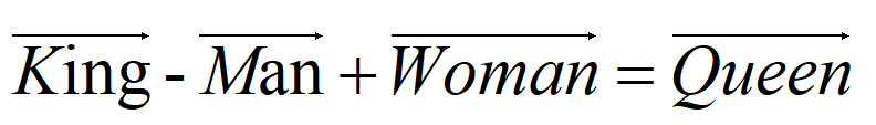
By removing the hidden layer and the activation function, we acknowledge that the relationships between several context words are also linearly correlated.Google’s Tomas Mkolov discovered that if the hidden layer in the DNN model is removed, the trained word vectors would be highly linearly correlated, leading to the remarkable property mentioned at the beginning of the previous article:
The second change addresses the reduction of the computational load of the original DNN’s softmax function. We changed the computation of softmax to finding the leaf nodes along a Huffman tree. In the Huffman tree, the non-leaf nodes are equivalent to the weights from the hidden layer to the output layer in the DNN. In the Huffman tree, we do not need to compute all non-leaf nodes; we only need to calculate the nodes along the path taken to find a specific leaf node, which greatly reduces the computational load.
2.5 Hierarchical Softmax Optimization Principle
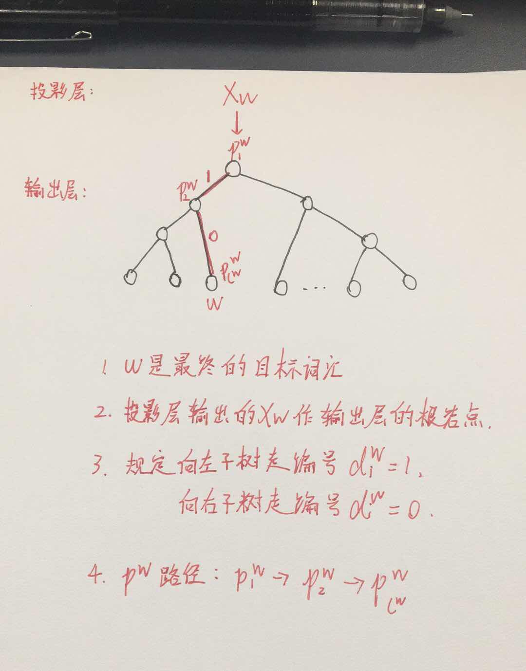
The above image shows a Huffman tree constructed based on word frequency, where each leaf node represents a word in the vocabulary. Before computation, let’s introduce some symbols:
Assume w is the target word we want to find, and Context(w) is the context words of the target word, with a total of c words.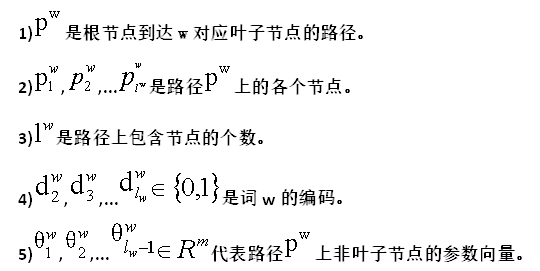
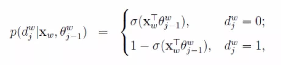
In word2vec, a binary logistic regression method is used, where the process from the root node to the leaf node is a binary classification problem. The probabilities of moving from the current node to the next node, along the left and right subtrees, are defined as:

Formula (1)
We use the sigmoid function to calculate the probability of selecting the current node. Since there are only two values, 0 and 1, we can express it in exponential form:

Formula (2)
Since the calculations for each non-leaf node are independent, the probability of finding the leaf node corresponding to the word w from the root node can be expressed as:
Formula (3)
Here, our objective function can be expressed as the log-likelihood:
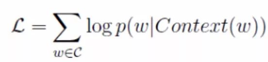
Formula (4)
Substituting (2) into (4) gives:
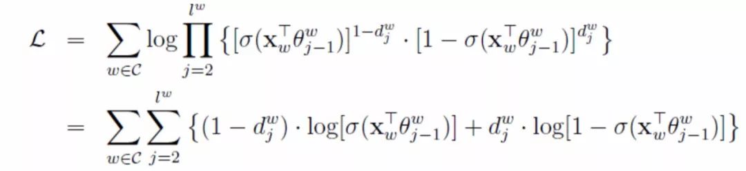
Formula (5)
For ease of understanding, we can express (5) as the sum of c terms:

Formula (6)
Our goal is to maximize the log-likelihood function (5), which is equivalent to maximizing each term in (6). At this point, we take the partial derivative of (6) with respect to each variable (X_w,θ_j-1) for each sample, substitute the partial derivative expression into the function to increase the gradient in the dimension corresponding to the partial derivative. This is the gradient ascent method.
Each term in (6) has two parameters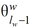 and X_w, and we take the partial derivative with respect to both parameters, starting with θ:

Formula (7)
The derivative of the sigmoid function is easy to calculate, and the final result for the derivative with respect to θ is:
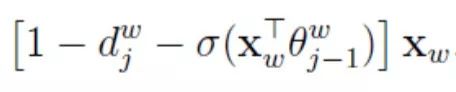
Formula (8)
Thus, the update expression for  is given by:
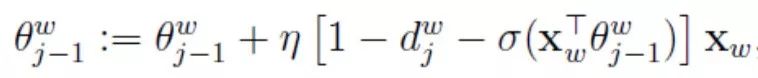
Formula (9)
Where  is a commonly used learning rate in machine learning, generally between 0 and 1. A larger value leads to faster training but may cause oscillations in local areas.
Similarly, taking the partial derivative with respect to X_w gives:
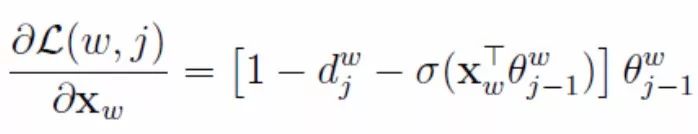
Formula (10)
Thus, we also obtain part of the update expression for X_w. Note that (10) is just the derivative of (6), which is only one term of the objective function (5). We still need to take the partial derivative of (5) for the other terms, and sum them up to get the complete derivative of X_w in (5). However, in the CBOW model of word2vec, X_w is the sum of the context word vectors, so we need to update the word vectors for each input word separately:
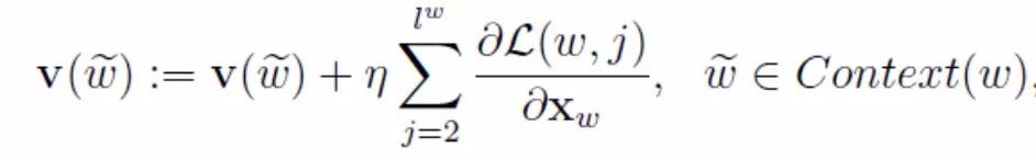
Formula (11)
Thus, we can obtain the pseudo-code for parameter updates. Before training starts, we need to input the vocabulary, count the frequency of each word to construct the Huffman tree, and then begin training:
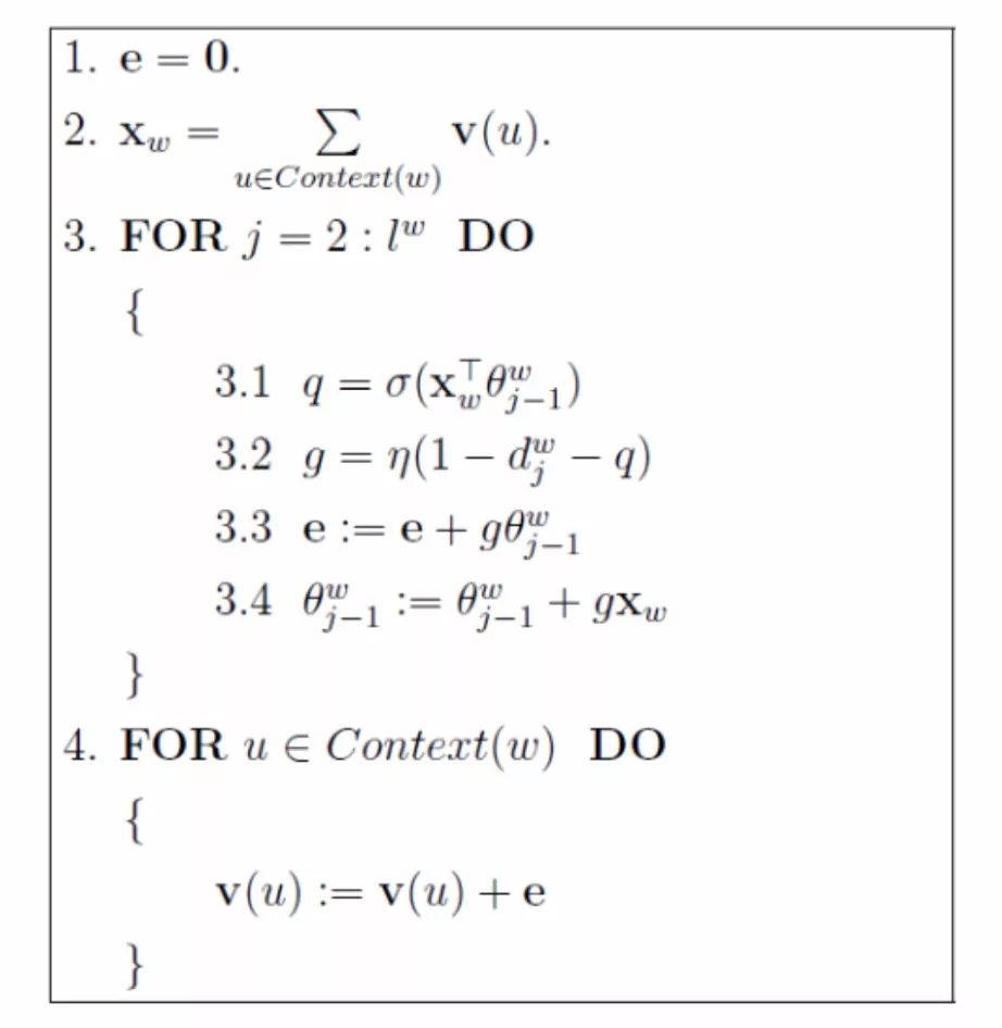
If the gradient converges, the gradient iteration ends, and the algorithm is complete.
3. Summary
Word2vec optimized by Hierarchical Softmax, compared to DNN, uses a Huffman tree network structure that does not require calculating all non-leaf nodes. Each time, it only backpropagates to update the parameters along the path on the tree, thus improving the efficiency of training word vectors. However, there are still some issues, such as the structure of the Huffman tree being based on a greedy approach, which is effective for training words with high frequency but less friendly for words with low frequency, resulting in deeper paths. The word2vec based on Negative Sampling can efficiently train low-frequency words. Next, we will continue to explain the last part of word2vec based on Negative Sampling. The learning journey is long, and I hope to share what I have learned about word2vec with everyone. If there are any shortcomings or misunderstandings, I welcome your guidance!

☟☟☟Click | Read the original text | View more exciting content