Summary of XGBoost Algorithm Principles

XGBoost (eXtreme Gradient Boosting) is known as extreme gradient boosting. It is the ace of ensemble learning methods, and most winners in Kaggle data mining competitions have used XGBoost. XGBoost performs exceptionally well in most regression and classification problems. This article provides a detailed introduction to the XGBoost algorithm principles.

The general method for constructing an optimal model is to minimize the loss function of the training data, denoted by the letter L, as shown below:

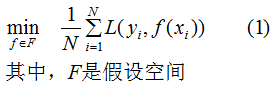
Equation (1) is called empirical risk minimization, and the model obtained from training has a high complexity. When the training data is small, the model is prone to overfitting.

Therefore, to reduce the model’s complexity, the following formula is often used:

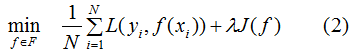
Where J(f) represents the model’s complexity, and Equation (2) is called structural risk minimization. Models that minimize structural risk often predict well on both training data and unknown test data.

Application: The generation and pruning of decision trees correspond to empirical risk minimization and structural risk minimization,XGBoost‘s decision tree generation is the result of structural risk minimization, which will be detailed later.

The Boosting method combines multiple weak learners to provide the final learning result. Regardless of whether the task is classification or regression, we use the regression idea to construct the optimal Boosting model.

Regression Idea: Treat the output of each weak learner as a continuous value, which allows for the accumulation of results from each weak learner and better utilization of the loss function to optimize the model.

Assuming is the output of the t-th weak learner, is the output of the model, and is the actual output, expressed as:

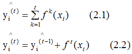
The above two equations represent an additive model, where it is assumed that the output of weak learners is continuous. Since the weak learners in regression tasks are inherently continuous, we will not discuss this further. Next, we will detail the regression idea in classification tasks.

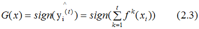
Regression Idea in Classification Tasks:

Based on the results of Equation 2.1, we obtain the final classifier:

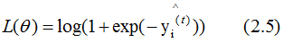
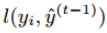
The loss function for classification generally chooses the exponential or logarithmic function. Here, we assume the loss function is the logarithmic function, with the learner’s loss function being:

If the actual output result yi=1, then:

Taking the gradient of Equation (2.5) with respect to gives:

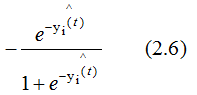
The negative gradient direction is the direction in which the loss function decreases the fastest. Since the value of Equation (2.6) is greater than 0, the weak learner iterates in the direction of increasing as shown in the graphic:

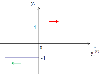
As shown in the figure above, when the actual label yi of the sample is 1, the model output result increases with the number of iterations (red line arrow), and the model’s loss function correspondingly decreases; when the actual label of the sample yi is -1, the model output result decreases with the number of iterations (red line arrow), and the model’s loss function correspondingly decreases.This is the principle of the additive model, which aims to reduce the loss function through multiple iterations.

Summary: The Boosting method treats the output of each weak learner as a continuous value, making the loss function a continuous value. Therefore, optimization of the model can be achieved through the iteration of weak learners, which is also the principle of the additive model in ensemble learning.

The objective function, i.e., the loss function, is constructed by minimizing the loss function to build the optimal model. From the first section, we know that the loss function should include a regularization term representing model complexity, and since the XGBoost model includes multiple CART trees, the model’s objective function is:

Equation (3.1) is the regularized loss function. The first part on the right side is the model’s training error, and the second part is the regularization term, which is the sum of the regularization terms of K trees.

Introduction to CART Trees:

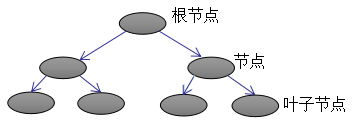
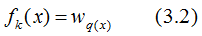
The above image represents the K-th CART tree. To determine a CART tree, two parts need to be defined: the first part is the structure of the tree, which maps input samples to a specific leaf node, denoted as. The second part is the values of each leaf node, where q(x) represents the output leaf node index, and represents the value corresponding to the leaf node index. By definition:

Definition of Tree Complexity

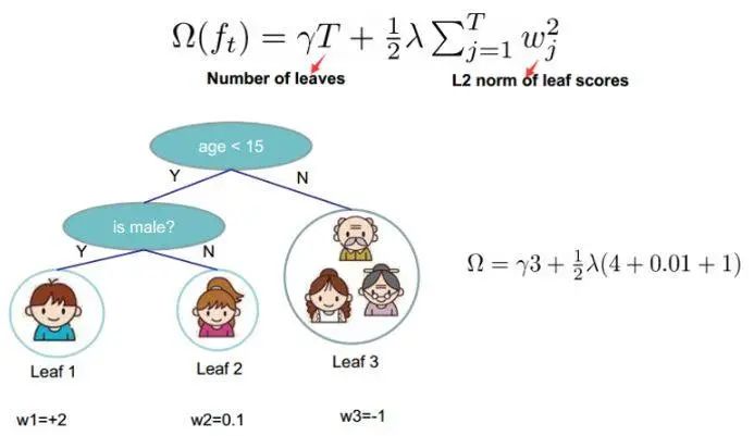
The XGBoost method corresponds to a model that includes multiple CART trees. The complexity of each tree is defined as:

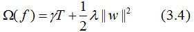
Where T is the number of leaf nodes, ||w|| is the norm of the leaf node vector. γ represents the difficulty of node splitting, and λ represents the L2 regularization coefficient.

As shown in the example, the complexity of the tree is represented as:

Derivation of the Objective Function

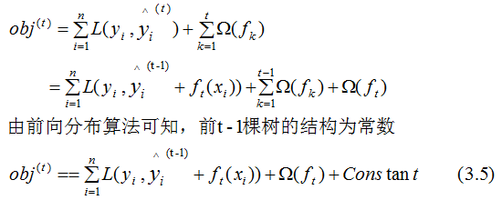
Based on Equation (3.1), the objective function of the learning model after t iterations is:

The second-order derivative approximation of Taylor’s formula is represented as:

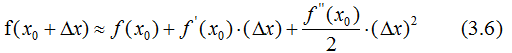
Let be Δx, then the second-order approximation of Equation (3.5) expands to:

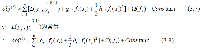
Where:

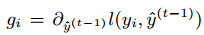
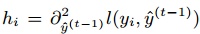
represents the prediction error of the learning model composed of the previous t-1 trees. gi and hi represent the first and second derivatives of the prediction error with respect to the current model, and the current model iterates in the direction that reduces the prediction error.

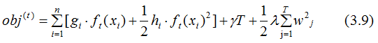
Ignoring the constant term in Equation (3.8), and combining with Equation (3.4), we get:

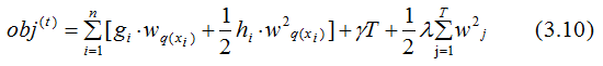
By simplifying Equation (3.9) with Equation (3.2):

The first part of Equation (3.10) is summed over all training samples, as all samples are mapped to the leaf nodes of the trees. We change our perspective and sum over all leaf nodes, yielding:

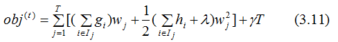
Let

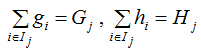Gj represents the sum of the first derivatives of all input samples mapped to leaf node j, and similarly, Hj represents the sum of the second derivatives.

Thus, we obtain:

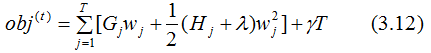
For a specific structure of the t-th CART tree (which can be represented by q(x)), its leaf nodes are independent of each other. Gj and Hj are determined quantities, thus Equation (3.12) can be regarded as a univariate quadratic function concerning the leaf nodes. Minimizing Equation (3.12) yields:

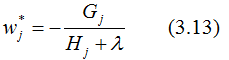
Thus, we obtain the final objective function:

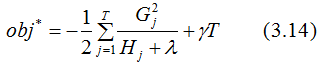
Equation (3.14) is also known as the scoring function, which is a standard for measuring the quality of the tree structure. The smaller the value, the better the structure. We use the scoring function to select the best split point, thus constructing the CART tree.

The scoring function derived in the previous section is a standard for measuring the quality of the tree structure. Therefore, we can use the scoring function to select the best split point. First, determine all split points of the sample features and evaluate each determined split point. The criteria for evaluating the split quality are as follows:

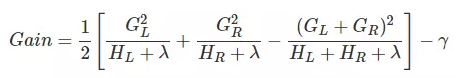
Gain represents the difference between the single-node obj* and the tree obj* of the two nodes after the split. By traversing all feature split points, the split point with the maximum Gain is the best split point. This method continues to split nodes to obtain the CART tree. If the γ value is set too high, Gain will be negative, indicating that the node should not be split since the tree structure worsens after the split. A higher γ value indicates stricter requirements for the decline in obj after splitting, and this value can be set in XGBoost.

1. XGBoost considers the complexity of the tree when generating CART trees, while GDBT does not; GDBT considers tree complexity during the tree pruning stage.

2. XGBoost fits the second-order derivative expansion of the previous round’s loss function, while GDBT fits the first-order derivative expansion of the previous round’s loss function. Therefore, XGBoost has higher accuracy and requires fewer iterations to achieve the same training effect.

3. XGBoost and GDBT both iteratively improve model performance, but XGBoost can utilize multithreading to select the best split point, significantly improving runtime speed.

PS: This section only selects a few differences relevant to this article.