
Hello everyone, today let’s talk about XGBoost ~
XGBoost (Extreme Gradient Boosting) is an ensemble learning algorithm that is an improvement of gradient boosting trees. It builds a powerful ensemble model by combining multiple weak learners (usually decision trees).
The core principle of XGBoost involves optimizing the loss function and constructing tree models.
Core Principles
1. Loss Function:
Assume we have a training dataset consisting of n samples, where x is the feature vector and y is the corresponding label.
XGBoost approximates the loss function using Taylor expansion. For a general loss function L, the Taylor expansion can be expressed as:
where ft is the current model’s prediction, gt and ht are the first-order derivative (gradient) and second-order derivative (Hessian matrix) of the loss function with respect to the prediction. Here, i indicates the i-th sample.
2. Regularization Term:
To prevent overfitting, XGBoost introduces a regularization term. The regularization term accounts for the complexity of the tree model and can be expressed as:
where k is the number of leaf nodes, w is the score of the leaf nodes, and λ and α are regularization parameters.
3. Objective Function:
The objective function of XGBoost is the weighted sum of the loss function and the regularization term. Assuming we have T tree models, each represented as ft, the objective function can be expressed as:
4. Model Update:
XGBoost uses a greedy algorithm to iteratively construct tree models. In each iteration, a new tree model is learned to minimize the objective function. The model update consists of two steps: leaf node splitting and leaf node weight updates.
For a leaf node j, its score wj can be calculated using the following formula:
where gj is the sum of the first-order gradients of all samples in leaf node j, and hj is the sum of the second-order gradients of all samples in leaf node j. Moreover, once the score of the leaf node is determined, an optimization algorithm (such as an approximate greedy algorithm) can be used to select the best split point.
5. Prediction:
The final model’s prediction results can be obtained by summing the output values of all trees:
where ft(x) represents the predicted output of the t-th tree for sample x.
In summary, XGBoost builds a powerful ensemble model by optimizing the objective function, iteratively constructing tree models, and optimizing the structure of the trees using a greedy algorithm.
Features and Applicable Scenarios
As an efficient ensemble learning algorithm, here are 7 notable features of XGBoost:
1. Efficient Parallel Processing:
-
XGBoost can effectively utilize multi-core processors for parallel computation, accelerating the model training process. -
It adopts a distributed computing framework, enabling quick training on large-scale datasets.
2. Highly Optimized Loss Function:
-
XGBoost uses Taylor expansion to approximate the loss function, allowing for better understanding of the data and faster convergence to the optimal solution. -
With first-order and second-order derivative information, XGBoost can estimate the loss of each sample more accurately.
3. Regularization and Pruning:
-
XGBoost controls the complexity of the model through the regularization term, preventing overfitting. -
It utilizes pruning techniques to reduce the size of the trees, lowering model complexity and improving generalization ability.
4. Scalability and Flexibility:
-
XGBoost can seamlessly integrate with various programming languages and data processing frameworks (such as Python, R, Spark). -
It supports custom loss functions and evaluation metrics, adapting to various tasks and needs.
5. Feature Importance Evaluation:
-
XGBoost provides an intuitive method to evaluate feature importance, assisting users in feature selection and model interpretation.
6. Handling Missing Values:
-
XGBoost can automatically handle missing values without requiring additional processing or filling.
7. Support for Multiple Objective Functions:
-
XGBoost supports various types of tasks such as classification, regression, and ranking, flexibly addressing different problems.
XGBoost is particularly effective in solving problems including but not limited to:
-
Classification Problems: XGBoost performs excellently in handling classification problems, effectively managing high-dimensional features and large-scale datasets. -
Regression Problems: For regression problems, XGBoost can provide accurate predictions and lower generalization error. -
Ranking Problems: In scenarios requiring ranking, such as search engines and recommendation systems, XGBoost can learn effective ranking models. -
Anomaly Detection: XGBoost can learn anomaly patterns for anomaly detection, applicable in financial fraud detection, industrial anomaly monitoring, etc. -
Feature Engineering: XGBoost can automatically handle missing and anomalous values, reducing the workload of feature engineering. -
Model Interpretation: XGBoost offers intuitive feature importance evaluation, helping to explain the model’s prediction results.
Complete Case Study
Below is a complete case study using the XGBoost algorithm for binary classification, including dataset, Python code, and result visualization. We will use the Iris dataset as an example, which contains four features and three classes.
Case Process
-
Data loading and preprocessing. -
Feature engineering and data splitting. -
Training the model using XGBoost. -
Model evaluation and visualization.
Dataset
We will use the Iris dataset, which contains 150 samples, each with four features: sepal length, sepal width, petal length, and petal width, along with a target variable representing the class of the iris flower (Setosa, Versicolor, and Virginica).
Code
import numpy as np
import pandas as pd
import xgboost as xgb
from sklearn.datasets import load_iris
from sklearn.model_selection import train_test_split
from sklearn.metrics import accuracy_score, confusion_matrix
import matplotlib.pyplot as plt
import seaborn as sns
from mpl_toolkits.mplot3d import Axes3D
# Load the Iris dataset
iris = load_iris()
X = iris.data
y = iris.target
# Data splitting
X_train, X_test, y_train, y_test = train_test_split(X, y, test_size=0.2, random_state=42)
# Set XGBoost parameters
param = {'max_depth': 3, 'eta': 0.3, 'objective': 'multi:softmax', 'num_class': 3}
num_round = 20
# Train the model
dtrain = xgb.DMatrix(X_train, label=y_train)
dtest = xgb.DMatrix(X_test, label=y_test)
bst = xgb.train(param, dtrain, num_round)
# Make predictions on the test set
y_pred = bst.predict(dtest)
# Calculate accuracy
accuracy = accuracy_score(y_test, y_pred)
print("Accuracy:", accuracy)
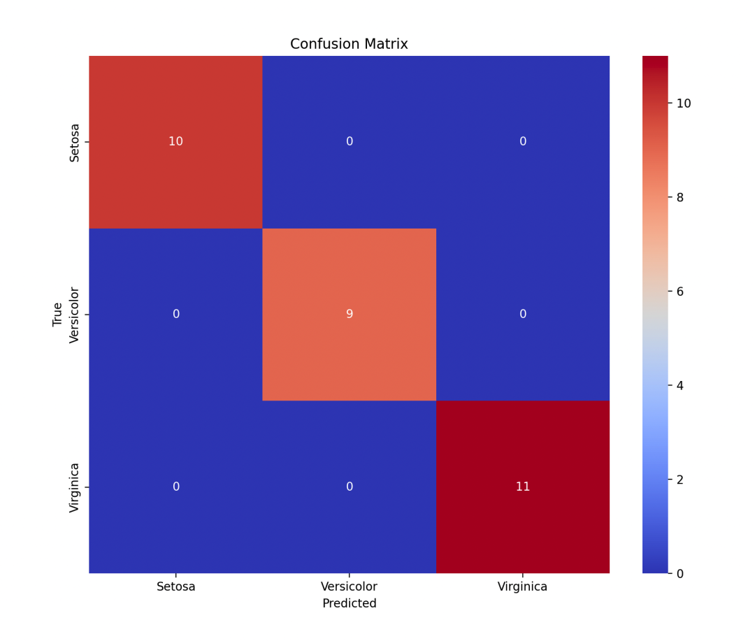
# Plot confusion matrix
labels = ['Setosa', 'Versicolor', 'Virginica']
cm = confusion_matrix(y_test, y_pred)
plt.figure(figsize=(10, 8))
sns.heatmap(cm, annot=True, fmt='d', cmap='coolwarm', xticklabels=labels, yticklabels=labels)
plt.xlabel('Predicted')
plt.ylabel('True')
plt.title('Confusion Matrix')
plt.show()
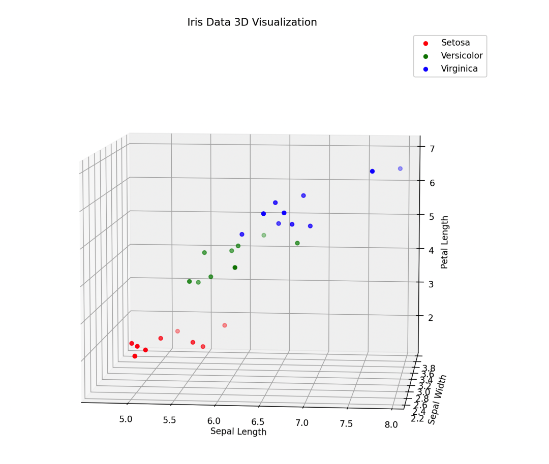
# 3D Visualization
fig = plt.figure(figsize=(12, 10))
ax = fig.add_subplot(111, projection='3d')
colors = ['r', 'g', 'b']
for i in range(3):
ax.scatter(X_test[y_test == i, 0], X_test[y_test == i, 1], X_test[y_test == i, 2], c=colors[i], label=labels[i])
ax.set_xlabel('Sepal Length')
ax.set_ylabel('Sepal Width')
ax.set_zlabel('Petal Length')
ax.set_title('Iris Data 3D Visualization')
plt.legend()
plt.show()In practical applications, you can adjust the parameters of XGBoost to achieve better performance, such as using cross-validation to select the best parameter combination.
Plotting the Confusion Matrix
Visualization
In Conclusion
XGBoost is an ensemble learning algorithm that builds powerful predictive models based on decision trees. It iteratively trains multiple decision tree models, continuously optimizing model performance using gradient boosting techniques. XGBoost performs excellently across various datasets and is widely used in classification and regression problems.
A simple and clear case every day; if you are interested in articles like this.
Feel free to follow, like, and share~