-
Concept of XGBoost
XGBoost stands for “Extreme Gradient Boosting”. The XGBoost algorithm is a type of ensemble algorithm formed by combining base functions with weights, resulting in a good fitting effect on data.
Unlike traditional Gradient Boosting Decision Trees (GBDT), XGBoost adds a regularization term to the loss function. Additionally, since some loss functions are difficult to compute derivatives for, XGBoost uses the second-order Taylor expansion of the loss function as the fitting of the loss function.
Due to its efficiency in handling large-scale datasets and complex models, along with excellent performance in preventing overfitting and improving generalization ability, XGBoost has become popular in statistics, data mining, and machine learning fields since its introduction.
2. Gradient Boosting Trees and Boosting Algorithms
XGBoost is based on the algorithm of gradient boosting trees, so it is essential to understand the principles of gradient boosting trees first.
Gradient boosting trees are an ensemble learning method that iteratively trains a series of weak learners (usually decision trees). Each iteration attempts to correct the errors from the previous iteration, ultimately combining these weak learners into a strong learner.
3. XGBoost Model Formula
For a dataset containing n samples with m dimensions, the XGBoost model can be expressed as:
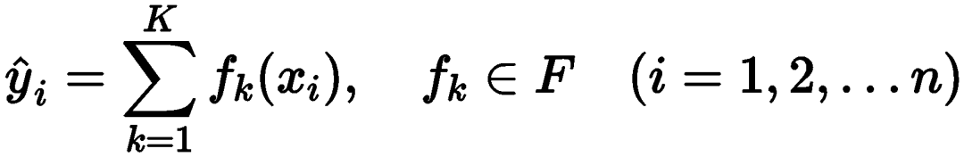
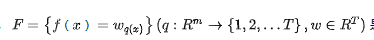
Where,
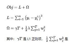
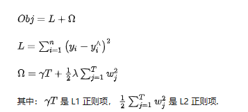
The objective function can be written as:
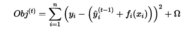
When optimizing the model with training data, it is necessary to keep the original model unchanged, adding a new function f to the model to minimize the objective function as much as possible. The specific process is as follows:

At this point, the objective function is expressed as:
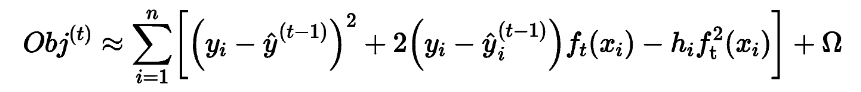
In the XGBoost algorithm, to quickly find the parameters that minimize the objective function, the second-order Taylor expansion of the objective function is performed, resulting in an approximate objective function:
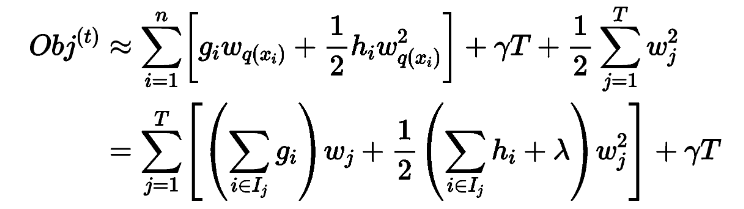
When the constant term is removed, it can be seen that the objective function is only related to the first and second derivatives of the error function. At this point, the objective function is expressed as:
If the tree structure part q is known, the objective function can be used to find the optimal Wj and obtain the optimal objective function value. Its essence can be reduced to solving the minimum value of a quadratic function. The solution is:
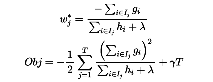
Obj can be used as a scoring function to evaluate the model; the smaller the Obj value, the better the model performance. By recursively calling the aforementioned tree-building method, a large number of regression tree structures can be obtained, and the optimal tree structure can be searched using Obj, which is then incorporated into the existing model to establish the optimal XGBoost model.
4. Case Study and Software Implementation
4.1 Case Introduction
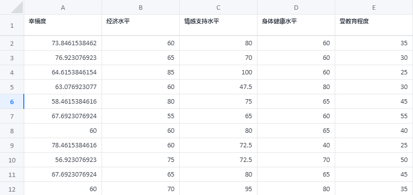
To study the factors influencing “happiness”, there are four variables that may affect happiness: economic income, education level, physical health, and emotional support. An XGBoost model is established to predict happiness.
4.2 Software Implementation
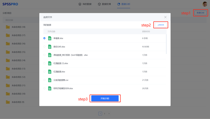
Step1: Open SPSSPRO and create a new analysis;
Step2: Upload the data;
Step3: Select the corresponding data, preview it, confirm it is correct, and click to start the analysis;
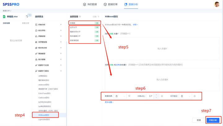
Step4: Select [XGBoost Regression];
Step5: Check the corresponding data format and input the [XGBoost Regression] data as required;
Step6: Set parameters (the parameters in “More Settings” can be set on the client);
Step7: Click [Start Analysis] to complete all operations.
4.3 Result Presentation
Output Result 1: Model Parameters
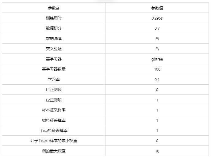
Chart Explanation: The table above shows the input parameters and the time taken for training the model.
Output Result 2: Feature Importance
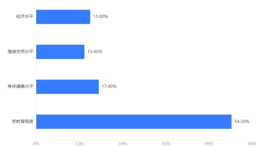
Chart Explanation: The above bar chart or table shows the importance ratio of each feature (independent variable). (Note: Sometimes, feature importance can be used to infer the value of that variable in real life, as this importance often determines the classification result.)
Analysis: The important factor determining the classification result in the XGBoost model is the education level.
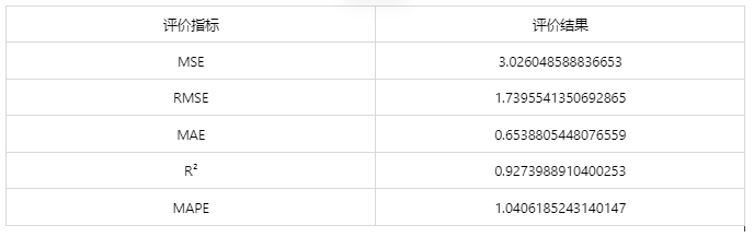
Output Result 3: Model Evaluation Results
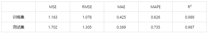
Chart Explanation: The table above displays the predictive evaluation metrics for the cross-validation set, training set, and testing set, measuring the predictive performance of XGBoost through quantitative metrics. Among them, the evaluation metrics of the cross-validation set can continuously adjust hyperparameters to obtain a reliable and stable model.
● MSE (Mean Squared Error): The expected value of the square of the difference between the predicted value and the actual value. The smaller the value, the higher the model accuracy.
● RMSE (Root Mean Squared Error): The square root of MSE; the smaller the value, the higher the model accuracy.
● MAE (Mean Absolute Error): The average of absolute errors, reflecting the actual situation of prediction errors. The smaller the value, the higher the model accuracy.
● MAPE (Mean Absolute Percentage Error): A transformation of MAE, expressed as a percentage. The smaller the value, the higher the model accuracy.
● R²: Compared to using only the mean for predictions, the closer the result is to 1, the higher the model accuracy.
Analysis: The R-squared value in the training set is 0.989, and in the testing set, it is 0.987, indicating excellent fitting performance.
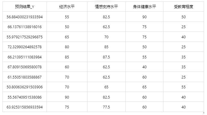
Output Result 4: Test Data Prediction Evaluation Results
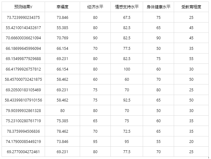
Chart Explanation: The table above shows the classification results of the XGBoost model on the test data; the first column is the predicted result, and the second column is the actual value of the dependent variable.
Output Result 5: Test Data Prediction Chart
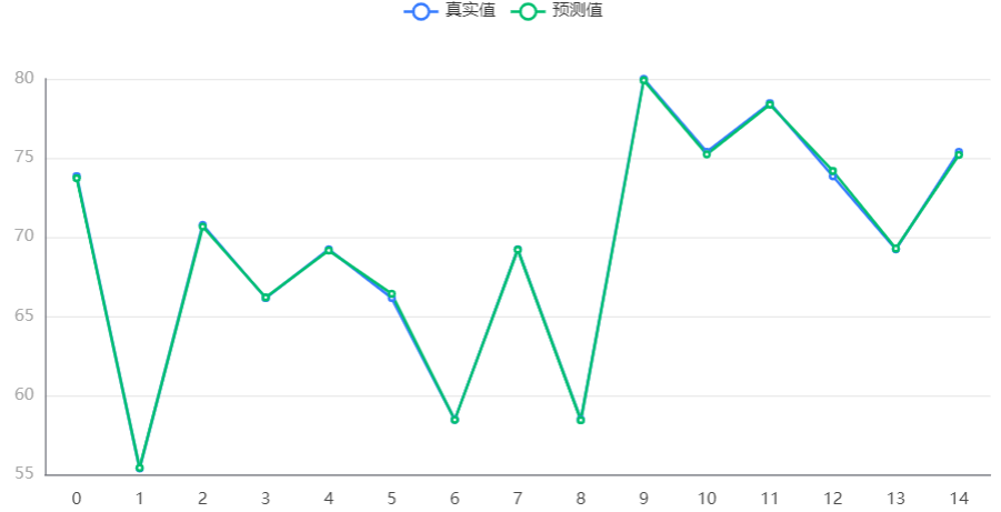
Chart Explanation: The above chart shows the prediction status of XGBoost on the test data. It can be seen that the actual values are very close to the predicted values, indicating that the trained XGBoost model has excellent predictive performance on the test set.
Output Result 6: Model Prediction and Application (This function is only supported in the client)
Note: When the prediction function cannot be performed, check whether there are categorical variables or missing values in the dataset:
● If there are categorical variables, please encode them in both the training dataset and the dataset used for prediction before proceeding.
(SPSSPRO: Data Processing -> Data Encoding -> Encode categorical variables into quantitative ones)
● If there are missing values in the dataset used for prediction, please remove the missing values before proceeding.
Situation 1: After the model evaluation above, if the model classification result is good and practical, we can apply this model. Click [Model Prediction] to upload the file and directly obtain the prediction results.

After the above operations, the following results are obtained:
Situation 2: If the uploaded data includes the actual values of the dependent variable, not only can you obtain the prediction results, but you can also get the current application data prediction evaluation effects.

After the above operations, the following results are obtained:
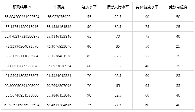
Since XGBoost has randomness, the results of each computation are different. If you need to save the trained model, you must use the SPSSPRO client.
5. Conclusion
From the previous introduction, we learned that the XGBoost regression model has several parameters that need to be specified by the designer, as well as some parameters that the model learns automatically. So, which parameters need to be determined by the model designer?
The hyperparameters of the XGBoost regression model need to be determined by the model designer, including learning rate, number of trees, maximum depth of trees, regularization parameters, etc. The choice of these hyperparameters has a significant impact on the model’s performance and generalization ability. The model designer needs to determine the optimal hyperparameter combination through experience, cross-validation, and grid search.
On the other hand, the XGBoost regression model will train according to the given hyperparameters using the gradient boosting tree algorithm and automatically learn ordinary parameters, such as tree structure, leaf node weights, etc. These parameters are adjusted and optimized automatically by the model based on the data, without manual specification.
However, determining the hyperparameters is a challenging task that requires practice and experimentation to find the best hyperparameter combination. It is hoped that designers can fully leverage the advantages of XGBoost regression through continuous efforts and exploration to achieve better model performance.
Editor / Zhang Zhihong
Reviewer / Fan Ruiqiang
Recheck / Zhang Zhihong
Click below
Follow us