Summary of Multi-GPU Parallel Training with PyTorch

Why Use Multi-GPU Parallel Training

In simple terms, there are two reasons: the first is that a model cannot fit on a single GPU, but can run completely on two or more GPUs (like the early AlexNet). The second is that parallel computation across multiple GPUs can speed up training. To become a “master alchemist”, mastering multi-GPU parallel training is an indispensable skill.

Common Multi-GPU Training Methods:

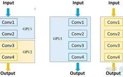
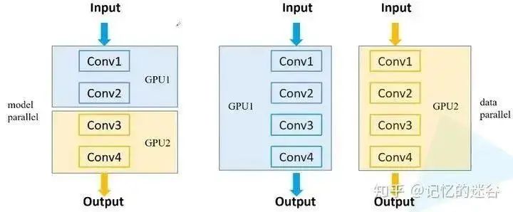
1. Model Parallelism: If the model is particularly large and cannot fit into the memory of a single GPU, different modules of the network need to be placed on different GPUs, allowing for the training of larger networks. (Left half of the image below)2. Data Parallelism: The entire model is placed on one GPU and then copied to each GPU, performing forward and backward propagation simultaneously. This effectively increases the batch size. (Right half of the image below)

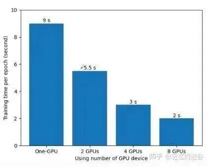
In the environment of pytorch1.7 + cuda10 + TeslaV100, using ResNet34, with batch_size=16, SGD trained on the flower dataset, the results are as follows: using one GPU takes 9 seconds per epoch, using two GPUs takes 5.5 seconds, and using eight GPUs takes 2 seconds. Here is a question: why is the running time not approximately 9/8 ≈ 1.1 seconds? Because as the number of GPUs increases, the communication between devices becomes more complex, so the speedup in training also diminishes with an increasing number of GPUs.

How Do Error Gradients Communicate Between Different Devices?

At the end of each training step on each GPU, the loss gradients from each GPU are averaged, rather than each GPU computing its own.

How Does Batch Normalization Synchronize Between Different Devices?

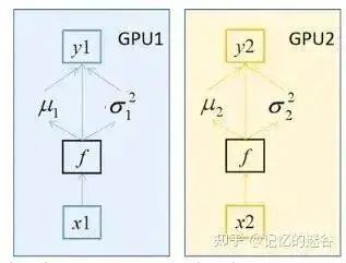
Assuming batch_size=2, the mean and variance computed by each GPU are based on these two samples. The property of Batch Normalization is that the larger the batch_size, the closer the mean and variance are to those of the entire dataset, resulting in better performance. When using multiple GPUs, the mean and variance for each Batch Normalization layer are calculated based on the inputs across all devices. If GPU1 and GPU2 both generate two feature layers respectively, then the two GPUs together compute the mean and variance for four feature layers, which can be considered as batch_size=4. Note: If Batch Normalization is not synchronized, and each device computes its own mean and variance for its batch of data, the effect will be the same as with a single GPU, only improving training speed; if synchronized Batch Normalization is used, there will be some improvement, but a portion of the parallel speed will be lost.

The image below shows the three scenarios of using a single GPU and whether synchronized Batch Normalization is used. It can be seen that using synchronized Batch Normalization (orange line) generally performs better than not using it (blue line), although the training time is longer. The performance of using a single GPU (black line) and not using synchronized Batch Normalization is similar.

Two GPU Training Methods: DataParallel and DistributedDataParallel:

• DataParallel is single-process multi-threaded and can only work on a single machine. DistributedDataParallel is multi-process and can work on a single machine or multiple machines.
• DataParallel is usually slower than DistributedDataParallel. Therefore, the mainstream method currently is DistributedDataParallel.

Common GPU Startup Methods in PyTorch:

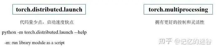
Note: If the distributed.launch method is manually terminated after starting training, it is best to check the memory usage, as there is a small probability that the process may not be killed, which will occupy some GPU memory resources.Next, based on the classification problem, we will detail the process of using DistributedDataParallel:First, initialize the environment for each process:

def init_distributed_mode(args):# If it's a multi-machine multi-GPU setup, WORLD_SIZE represents the number of machines used, RANK corresponds to which machine# If it's a single machine multi-GPU setup, WORLD_SIZE represents how many GPUs there are, RANK and LOCAL_RANK represent which GPU    if 'RANK' in os.environ and 'WORLD_SIZE' in os.environ:        args.rank = int(os.environ["RANK"])        args.world_size = int(os.environ['WORLD_SIZE'])# LOCAL_RANK represents which GPU on a certain machine        args.gpu = int(os.environ['LOCAL_RANK'])    elif 'SLURM_PROCID' in os.environ:        args.rank = int(os.environ['SLURM_PROCID'])        args.gpu = args.rank % torch.cuda.device_count()else:        print('Not using distributed mode')        args.distributed = False    args.distributed = True    torch.cuda.set_device(args.gpu)  # Specify the GPU to be used for the current process    args.dist_backend = 'nccl'# Communication backend, recommended to use NCCL for NVIDIA GPUs    dist.barrier()  # Wait for each GPU to finish this part before continuing

In the initial stage of the main function, perform the following initialization operations. Note that the learning rate needs to be increased based on the number of GPUs used. Here, a simple multiplication method is used.

def main(args):if torch.cuda.is_available() is False:raise EnvironmentError("not find GPU device for training.")    # Initialize the environment for each processinit_distributed_mode(args=args)rank = args.rankdevice = torch.device(args.device)batch_size = args.batch_sizenum_classes = args.num_classesweights_path = args.weightsargs.lr *= args.world_size  # The learning rate needs to be multiplied by the number of parallel GPUs

Instantiating the dataset can use the same method as with a single GPU, but when sampling the samples, unlike a single machine, it requires using DistributedSampler and BatchSampler.

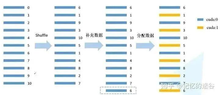
# Assign training sample indices corresponding to each ranktrain_sampler=torch.utils.data.distributed.DistributedSampler(train_data_set)val_sampler=torch.utils.data.distributed.DistributedSampler(val_data_set)# Group every batch_size elements into a listtrain_batch_sampler=torch.utils.data.BatchSampler(train_sampler,batch_size,drop_last=True)

The principle of DistributedSampler is illustrated in the image: assuming the current dataset has samples indexed from 0 to 10 (11 samples total), using 2 GPUs for computation. First, shuffle the data order, then calculate 11/2 = 6 (rounding up), then multiply by the number of GPUs (2) to get 12. Since there are only 11 data points, the first data point (index 6) is repeated at the end, resulting in 12 data points that can be evenly distributed to each GPU. Then, the data is distributed: the data is assigned to different GPUs at intervals.

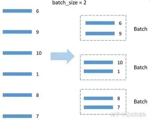
The principle of BatchSampler: DistributedSampler distributes the data to two GPUs. Taking the first GPU as an example, the data assigned is 6, 9, 10, 1, 8, 7. Assuming batch_size=2, the data is grouped in pairs. During training, each time a batch of data is fetched, it is taken from the organized batches. Note: Only the training set is processed; the validation set does not use BatchSampler.

Next, use the defined dataset and sampler methods to load the data:

train_loader = torch.utils.data.DataLoader(train_data_set,batch_sampler=train_batch_sampler,pin_memory=True,   # Load directly into memory for accelerationnum_workers=nw,collate_fn=train_data_set.collate_fn)val_loader = torch.utils.data.DataLoader(val_data_set,batch_size=batch_size,sampler=val_sampler,pin_memory=True,num_workers=nw,collate_fn=val_data_set.collate_fn)

If there are pre-trained weights, ensure that each GPU loads the weights identically. The main process should save the model’s initialized weights, and other processes should load the weights saved by the main process. This ensures that the weights loaded on each GPU are consistent:

# Instantiate model    model = resnet34(num_classes=num_classes).to(device)# If pre-trained weights exist, load themif os.path.exists(weights_path):        weights_dict = torch.load(weights_path, map_location=device)# Simple comparison of the number of weight parameters for each layer        load_weights_dict = {k: v for k, v in weights_dict.items()if model.state_dict()[k].numel() == v.numel()}        model.load_state_dict(load_weights_dict, strict=False)else:        checkpoint_path = os.path.join(tempfile.gettempdir(), "initial_weights.pt")# If pre-trained weights do not exist, save the weights from the first process, then load them in other processes to maintain weight consistencyif rank == 0:            torch.save(model.state_dict(), checkpoint_path)        dist.barrier()# Note: Be sure to specify the map_location parameter, otherwise the first GPU may occupy more resources        model.load_state_dict(torch.load(checkpoint_path, map_location=device))

If model weights need to be frozen, it is basically the same as with a single GPU. If weights do not need to be frozen, you can choose whether to use synchronized Batch Normalization. Then wrap the model into a DDP model for easy communication between processes. The optimizer settings for multi-GPU and single-GPU are the same, and will not be elaborated here.

# Whether to freeze weightsif args.freeze_layers:for name, para in model.named_parameters():# Freeze all weights except the last fully connected layer            if "fc" not in name:                para.requires_grad_(False)else:# Only use SyncBatchNorm when training networks with BN structureif args.syncBN:# Training with SyncBatchNorm will take longer            model = torch.nn.SyncBatchNorm.convert_sync_batchnorm(model).to(device)# Convert to DDP model         model = torch.nn.parallel.DistributedDataParallel(model, device_ids=[args.gpu])# optimizer using SGD + cosine annealing strategy    pg = [p for p in model.parameters() if p.requires_grad]    optimizer = optim.SGD(pg, lr=args.lr, momentum=0.9, weight_decay=0.005)    lf = lambda x: ((1 + math.cos(x * math.pi / args.epochs)) / 2) * (1 - args.lrf) + args.lrf  # cosine    scheduler = lr_scheduler.LambdaLR(optimizer, lr_lambda=lf)

Differences from single GPU: the line train_sampler.set_epoch(epoch) will obtain a different generator during each iteration. Before starting to iterate each round, set a random seed by changing the epoch parameter passed in to shuffle the data order. By setting different random seeds, different GPUs can obtain different data each round. The subsequent parts are the same as with a single GPU.

for epoch in range(args.epochs):train_sampler.set_epoch(epoch)  mean_loss = train_one_epoch(model=model,optimizer=optimizer,data_loader=train_loader,device=device,epoch=epoch)scheduler.step()sum_num = evaluate(model=model,data_loader=val_loader,device=device)acc = sum_num / val_sampler.total_size

Let’s take a detailed look at the differences in training at each epoch (the above train_one_epoch).

def train_one_epoch(model, optimizer, data_loader, device, epoch):    model.train()    loss_function = torch.nn.CrossEntropyLoss()    mean_loss = torch.zeros(1).to(device)    optimizer.zero_grad()# Print training progress in process 0if is_main_process():        data_loader = tqdm(data_loader)for step, data in enumerate(data_loader):        images, labels = data        pred = model(images.to(device))        loss = loss_function(pred, labels.to(device))        loss.backward()        loss = reduce_value(loss, average=True)  #  In single GPU this does not apply, in multi-GPU, get the mean of the loss from all GPUs.        mean_loss = (mean_loss * step + loss.detach()) / (step + 1)  # update mean losses# Print average loss in process 0if is_main_process():            data_loader.desc = "[epoch {}] mean loss {}".format(epoch, round(mean_loss.item(), 3))        if not torch.isfinite(loss):            print('WARNING: non-finite loss, ending training ', loss)            sys.exit(1)        optimizer.step()        optimizer.zero_grad()# Wait for all processes to finish calculationsif device != torch.device("cpu"):        torch.cuda.synchronize(device)return mean_loss.item()

Next, let’s look at the evaluation phase, where the biggest difference from a single GPU is in the area of counting correctly predicted samples.

@torch.no_grad()def evaluate(model, data_loader, device):    model.eval()# Store the number of correctly predicted samples, each GPU will calculate its own correct sample count    sum_num = torch.zeros(1).to(device)# Print validation progress in process 0if is_main_process():        data_loader = tqdm(data_loader)for step, data in enumerate(data_loader):        images, labels = data        pred = model(images.to(device))        pred = torch.max(pred, dim=1)[1]        sum_num += torch.eq(pred, labels.to(device)).sum()# Wait for all processes to finish calculationsif device != torch.device("cpu"):        torch.cuda.synchronize(device)    sum_num = reduce_value(sum_num, average=False)  # Count of correctly predicted samplesreturn sum_num.item()

It is important to note that saving the model weights should be done in the main process.

if rank == 0:print("[epoch {}] accuracy: {}".format(epoch, round(acc, 3)))            tags = ["loss", "accuracy", "learning_rate"]            tb_writer.add_scalar(tags[0], mean_loss, epoch)            tb_writer.add_scalar(tags[1], acc, epoch)            tb_writer.add_scalar(tags[2], optimizer.param_groups[0]["lr"], epoch)            torch.save(model.module.state_dict(), "./weights/model-{}.pth".format(epoch))

If training from scratch, the initialized weights generated by the main process are saved as temporary files, which should be removed after training is completed. Finally, the process group needs to be dismantled.

if rank == 0:# Delete temporary cache file        if os.path.exists(checkpoint_path) is True:            os.remove(checkpoint_path)    dist.destroy_process_group()  # Dismantle the process group, releasing resources