
Click the above “Beginner Learning Vision“, select to add “Star” or “Top“
Essential knowledge delivered promptly
1. IntroductionDeep Convolutional Neural Networks have greatly changed the research landscape of image classification [1]. As more layers are added, the model’s expressive power increases; it can learn more complex representations. To some extent, there seems to be a positive correlation between the depth of the network and the accuracy of the model. On the other hand, as the network deepens, the vanishing/exploding gradient problem becomes more severe. Normalized initialization and normalization layers eventually solved this issue, and deep networks began to converge. However, contrary to the intuitive reasoning before subsequent experiments, as the depth increases, the accuracy of the model starts to saturate and then actually decreases rapidly. This is not due to overfitting but rather the limitations of the current solvers used to optimize the model [2].The introduction of ResNet addresses the degradation problem [2]. It introduces a systematic way to use skip connections, which connect layers by skipping one or more layers. These short connections simply perform identity mappings, and their outputs are added to the outputs of the stacked layers (which does not increase additional parameters or computational complexity). The idea behind this is that if multiple nonlinear layers can asymptotically approximate complex functions (still theoretically researched, but foundational to deep learning), then the residual function could potentially do the same. The advantage is that it simplifies the work of the solver at the same time. Other types of connections, such as scaling and 1×1 convolutional skip connections, were studied in [3].Our task is to classify a series of labeled images.We want to compare the accuracy of two different methods; the first is the classic Convolutional Neural Network, and the second is the Residual Network. Our goal is to demonstrate the power of the Residual Network, even in not very deep networks.This is a good method to help optimize the process while addressing the degradation problem. We experimentally tested the Residual Network and found that it is easier to overfit. To address this issue, we adopted a data augmentation strategy to comprehensively augment the dataset.We used the Simpsons character dataset [4]. We only filtered the dataset to include classes with over 100 images (characters). After splitting the training, validation, and test datasets, the results of the dataset sizes are as follows: 12411 images for training, 3091 images for validation, and 950 images for testing.Code and data are also available as usual on my GitHub.https://github.com/luisroque/deep-learning-articles
2. Data Preprocessing
We created generators to provide data to the model. We also applied a transformation to normalize the data, split the data between the training and validation datasets, and defined a batch size of 32 (see [5] for better understanding of preprocessing and generators).
import tensorflow as tf
from tensorflow.keras.models import Model
from tensorflow.keras.layers import Layer, BatchNormalization, Conv2D, Dense, Flatten, Add, Dropout, BatchNormalization
import numpy as np
from tensorflow.keras.datasets import fashion_mnist
from tensorflow.keras.utils import to_categorical
import matplotlib.pyplot as plt
from sklearn.model_selection import train_test_split
from tensorflow.keras.preprocessing.image import ImageDataGenerator
import os
from tensorflow.keras import Input, layers
from tensorflow.keras.layers import Dense, Flatten, Conv2D, MaxPooling2D
import time

directory_train = "./simpsons_data_split/train/"
directory_test = "./simpsons_data_split/test/"

def get_ImageDataGenerator(validation_split=None):
    image_generator = ImageDataGenerator(rescale=(1/255.),
                                         validation_split=validation_split)
    return image_generator

image_gen_train = get_ImageDataGenerator(validation_split=0.2)

def get_generator(image_data_generator, directory, train_valid=None, seed=None):
    train_generator = image_data_generator.flow_from_directory(directory,
                                                               batch_size=32,
                                                                 class_mode='categorical',
                                                               target_size=(128,128),
                                                               subset=train_valid,
                                                               seed=seed)
    return train_generator

train_generator = get_generator(image_gen_train, directory_train, train_valid='training', seed=1)
validation_generator = get_generator(image_gen_train, directory_train, train_valid='validation')

Found 12411 images belonging to 19 classes.
Found 3091 images belonging to 19 classes.
We also created an augmented dataset by applying a set of geometric and photometric transformations to reduce the likelihood of overfitting.Geometric transformations alter the geometric structure of images, keeping CNN invariant to position and orientation. Photometric transformations adjust the color channels of images, keeping CNN invariant to changes in color and lighting.
def get_ImageDataGenerator_augmented(validation_split=None):
    image_generator = ImageDataGenerator(rescale=(1/255.),
                                        rotation_range=40,
                                        width_shift_range=0.2,
                                        height_shift_range=0.2,
                                        shear_range=0.2,
                                        zoom_range=0.1,
                                        brightness_range=[0.8,1.2],
                                        horizontal_flip=True,
                                        validation_split=validation_split)
    return image_generator

image_gen_train_aug = get_ImageDataGenerator_augmented(validation_split=0.2)
train_generator_aug = get_generator(image_gen_train_aug, directory_train, train_valid='training', seed=1)
validation_generator_aug = get_generator(image_gen_train_aug, directory_train, train_valid='validation')

Found 12411 images belonging to 19 classes.
Found 3091 images belonging to 19 classes.
We can iterate through the generator to get a batch of images equal to the batch size defined above.
target_labels = next(os.walk(directory_train))[1]

target_labels.sort()

batch = next(train_generator)
batch_images = np.array(batch[0])
batch_labels = np.array(batch[1])
target_labels = np.asarray(target_labels)

plt.figure(figsize=(15,10))
for n, i in enumerate(np.arange(10)):
    ax = plt.subplot(3,5,n+1)
    plt.imshow(batch_images[i])
    plt.title(target_labels[np.where(batch_labels[i]==1)[0][0]])
    plt.axis('off')

3. Benchmark Model
We defined a simple CNN as a benchmark model.It uses 2D convolutional layers (performing spatial convolutions on images) and max pooling operations. Followed by a Dense layer with 128 units and ReLU activation, along with a Dropout layer with a rate of 0.5. Finally, the last layer produces the output of our network, with the number of units equal to the number of target labels and using the softmax activation function.The model is compiled using the Adam optimizer with default settings and categorical cross-entropy loss.
def get_benchmark_model(input_shape):
    x = Input(shape=input_shape)
    h = Conv2D(32, padding='same', kernel_size=(3,3), activation='relu')(x)
    h = Conv2D(32, padding='same', kernel_size=(3,3), activation='relu')(x)
    h = MaxPooling2D(pool_size=(2,2))(h)
    h = Conv2D(64, padding='same', kernel_size=(3,3), activation='relu')(h)
    h = Conv2D(64, padding='same', kernel_size=(3,3), activation='relu')(h)
    h = MaxPooling2D(pool_size=(2,2))(h)
    h = Conv2D(128, kernel_size=(3,3), activation='relu')(h)
    h = Conv2D(128, kernel_size=(3,3), activation='relu')(h)
    h = MaxPooling2D(pool_size=(2,2))(h)
    h = Flatten()(h)
    h = Dense(128, activation='relu')(h)
    h = Dropout(.5)(h)
    output = Dense(target_labels.shape[0], activation='softmax')(h)

    model = tf.keras.Model(inputs=x, outputs=output)

    model.compile(optimizer='adam',
             loss='categorical_crossentropy',
             metrics=['accuracy'])
    return model

benchmark_model = get_benchmark_model((128, 128, 3))
benchmark_model.summary()

Model: "model"
_________________________________________________________________
Layer (type)                 Output Shape              Param #
=================================================================
input_1 (InputLayer)         [(None, 128, 128, 3)]     0
_________________________________________________________________
conv2d_1 (Conv2D)            (None, 128, 128, 32)      896
_________________________________________________________________
max_pooling2d (MaxPooling2D) (None, 64, 64, 32)        0
_________________________________________________________________
conv2d_2 (Conv2D)            (None, 64, 64, 64)        18496
_________________________________________________________________
conv2d_3 (Conv2D)            (None, 64, 64, 64)        36928
_________________________________________________________________
max_pooling2d_1 (MaxPooling2 (None, 32, 32, 64)        0
_________________________________________________________________
conv2d_4 (Conv2D)            (None, 30, 30, 128)       73856
_________________________________________________________________
conv2d_5 (Conv2D)            (None, 28, 28, 128)       147584
_________________________________________________________________
max_pooling2d_2 (MaxPooling2 (None, 14, 14, 128)       0
_________________________________________________________________
flatten (Flatten)            (None, 25088)             0
_________________________________________________________________
dense (Dense)                (None, 128)               3211392
_________________________________________________________________
dropout (Dropout)            (None, 128)               0
_________________________________________________________________
dense_1 (Dense)              (None, 19)                2451
=================================================================
Total params: 3,491,603
Trainable params: 3,491,603
Non-trainable params: 0
_________________________________________________________________

def train_model(model, train_gen, valid_gen, epochs):
    train_steps_per_epoch = train_gen.n // train_gen.batch_size
    val_steps = valid_gen.n // valid_gen.batch_size

    earlystopping = tf.keras.callbacks.EarlyStopping(patience=3)
    history = model.fit(train_gen,
                        steps_per_epoch = train_steps_per_epoch,
                        epochs=epochs,
                        validation_data=valid_gen,
                        callbacks=[earlystopping])

    return history

train_generator = get_generator(image_gen_train, directory_train, train_valid='training')
validation_generator = get_generator(image_gen_train, directory_train, train_valid='validation')
history_benchmark = train_model(benchmark_model, train_generator, validation_generator, 50)

Found 12411 images belonging to 19 classes.
Found 3091 images belonging to 19 classes.

Epoch 1/50
387/387 [==============================] - 139s 357ms/step - loss: 2.7674 - accuracy: 0.1370 - val_loss: 2.1717 - val_accuracy: 0.3488
Epoch 2/50
387/387 [==============================] - 136s 352ms/step - loss: 2.0837 - accuracy: 0.3757 - val_loss: 1.7546 - val_accuracy: 0.4940
Epoch 3/50
387/387 [==============================] - 130s 335ms/step - loss: 1.5967 - accuracy: 0.5139 - val_loss: 1.3483 - val_accuracy: 0.6102
Epoch 4/50
387/387 [==============================] - 130s 335ms/step - loss: 1.1952 - accuracy: 0.6348 - val_loss: 1.1623 - val_accuracy: 0.6619
Epoch 5/50
387/387 [==============================] - 130s 337ms/step - loss: 0.9164 - accuracy: 0.7212 - val_loss: 1.0813 - val_accuracy: 0.6907
Epoch 6/50
387/387 [==============================] - 130s 336ms/step - loss: 0.7270 - accuracy: 0.7802 - val_loss: 1.0241 - val_accuracy: 0.7240
Epoch 7/50
387/387 [==============================] - 130s 336ms/step - loss: 0.5641 - accuracy: 0.8217 - val_loss: 0.9674 - val_accuracy: 0.7438
Epoch 8/50
387/387 [==============================] - 130s 336ms/step - loss: 0.4496 - accuracy: 0.8592 - val_loss: 1.0701 - val_accuracy: 0.7441
Epoch 9/50
387/387 [==============================] - 130s 336ms/step - loss: 0.3677 - accuracy: 0.8758 - val_loss: 0.9796 - val_accuracy: 0.7645
Epoch 10/50
387/387 [==============================] - 130s 336ms/step - loss: 0.3041 - accuracy: 0.8983 - val_loss: 1.0681 - val_accuracy: 0.7561
4. ResNet
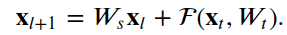
The deep residual network consists of many stacked units, which can be defined as:
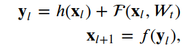
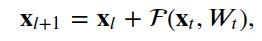
where x_l and x_{l+1} are the input and output of the l-th unit, F is the residual function, h(x_l) is the identity mapping, and F is the activation function. W_t is a set of weights (and biases) associated with the l-th residual unit.The number of layers proposed in [2] is 2 or 3. We define F as a stack of two 3×3 convolutional layers. In [2], f is the ReLU function applied after element-wise addition. We followed the architecture proposed later in [3], where f is simply an identity mapping. In this case,

We can write as,
or more generally written as,
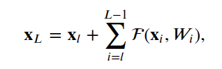
For any deeper unit L and shallower unit L. The features are
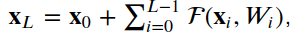
For any deep unit, L is the sum of the outputs of all previous residual functions plus x_0.In terms of the optimization process, backpropagation provides some intuition about why this type of connection helps the optimization process. We can write:
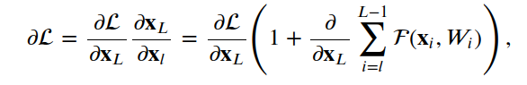
where L is the loss function, and note the gradient

and the term
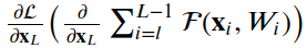
propagates through the weight layers. It can be shown that using this form, even when the weights are arbitrarily small, the gradients of the layers do not vanish.
4.1 Residual Unit
We use layer subclassing to build the residual unit. The custom layer class has three methods:<span>__init__</span>, <span>build</span> and <span>call</span>.<span>__init__</span> method calls the base layer class initializer using defined keyword arguments. The build method creates the layer. In our case, we define two sets of BatchNormalization, followed by Conv2D layers, and finally a set using the same number of filters as the layer input.The call method processes the input through the layer. In our case, we have the following order: first BatchNormalization, ReLu activation function, first Conv2D, second BatchNormalization, another ReLu activation function, and second Conv2D. Finally, we add the input to the output of the second Conv2D layer.
class ResidualUnit(Layer):
    def __init__(self, **kwargs):
        super(ResidualUnit, self).__init__(**kwargs)

    def build(self, input_shape):
        self.bn_1 = tf.keras.layers.BatchNormalization(input_shape=input_shape)
        self.conv2d_1 = tf.keras.layers.Conv2D(input_shape[3], (3, 3), padding='same')
        self.bn_2 = tf.keras.layers.BatchNormalization()
        self.conv2d_2 = tf.keras.layers.Conv2D(input_shape[3], (3, 3), padding='same')

    def call(self, inputs, training=False):
        x = self.bn_1(inputs, training)
        x = tf.nn.relu(x)
        x = self.conv2d_1(x)
        x = self.bn_2(x, training)
        x = tf.nn.relu(x)
        x = self.conv2d_2(x)
        x = tf.keras.layers.add([inputs, x])
        return x

test_model = tf.keras.Sequential([ResidualUnit(input_shape=(128, 128, 3), name="residual_unit")])
test_model.summary()

Model: "sequential"
_________________________________________________________________
Layer (type)                 Output Shape              Param #
=================================================================
residual_unit (ResidualUnit) (None, 128, 128, 3)       192
=================================================================
Total params: 192
Trainable params: 180
Non-trainable params: 12
_________________________________________________________________
4.2 Residual Unit with Increased Dimensions
In the architecture proposed in [2], there are residual units that increase dimensions. This is achieved by using a linear projection of the shortcut connection to match the required size:
In this case, it is accomplished by a 1×1 convolutional layer.
class FiltersChangeResidualUnit(Layer):

    def __init__(self, out_filters, **kwargs):
        super(FiltersChangeResidualUnit, self).__init__(**kwargs)
        self.out_filters = out_filters

    def build(self, input_shape):
        number_filters = input_shape[0]
        self.bn_1 = tf.keras.layers.BatchNormalization(input_shape=input_shape)
        self.conv2d_1 = tf.keras.layers.Conv2D(input_shape[3], (3, 3), padding='same')
        self.bn_2 = tf.keras.layers.BatchNormalization()
        self.conv2d_2 = tf.keras.layers.Conv2D(self.out_filters, (3, 3), padding='same')
        self.conv2d_3 = tf.keras.layers.Conv2D(self.out_filters, (1, 1))

    def call(self, inputs, training=False):
        x = self.bn_1(inputs, training)
        x = tf.nn.relu(x)
        x = self.conv2d_1(x)
        x = self.bn_2(x, training)
        x = tf.nn.relu(x)
        x = self.conv2d_2(x)
        x_1 = self.conv2d_3(inputs)
        x = tf.keras.layers.add([x, x_1])
        return x

test_model = tf.keras.Sequential([FiltersChangeResidualUnit(16, input_shape=(32, 32, 3), name="fc_resnet_unit")])
test_model.summary()

Model: "sequential_1"
_________________________________________________________________
Layer (type)                 Output Shape              Param #
=================================================================
fc_resnet_unit (FiltersChang (None, 32, 32, 16)        620
=================================================================
Total params: 620
Trainable params: 608
Non-trainable params: 12
_________________________________________________________________
4.3 Model
Finally, we can construct the complete model.We first define a Conv2D layer with 32 filters, a 7×7 kernel, and a stride of 2.After the first layer, we add residual units. Then, we add a new Conv2D layer with 32 filters, a 3×3 kernel, and a stride of 2.Next, we add residual units, allowing for dimensional changes to 64. To finalize our model, we flatten the data and feed it into a Dense layer with the softmax activation function and the same number of units as the classes.
class ResNetModel(Model):

    def __init__(self, **kwargs):
        super(ResNetModel, self).__init__()
        self.conv2d_1 = tf.keras.layers.Conv2D(32, (7, 7), strides=(2,2))
        self.resb = ResidualUnit()
        self.conv2d_2 = tf.keras.layers.Conv2D(32, (3, 3), strides=(2,2))
        self.filtersresb = FiltersChangeResidualUnit(64)
        self.flatten_1 = tf.keras.layers.Flatten()
        self.dense_o = tf.keras.layers.Dense(target_labels.shape[0], activation='softmax')

    def call(self, inputs, training=False):
        x = self.conv2d_1(inputs)
        x = self.resb(x, training)
        x = self.conv2d_2(x)
        x = self.filtersresb(x, training)
        x = self.flatten_1(x)
        x = self.dense_o(x)

        return x
resnet_model = ResNetModel()
resnet_model(inputs= tf.random.normal((32, 128,128,3)))
resnet_model.summary()

Model: "res_net_model"
_________________________________________________________________
Layer (type)                 Output Shape              Param #
=================================================================
conv2d_6 (Conv2D)            multiple                  4736
_________________________________________________________________
residual_unit (ResidualUnit) multiple                  18752
_________________________________________________________________
conv2d_7 (Conv2D)            multiple                  9248
_________________________________________________________________
filters_change_residual_unit multiple                  30112
_________________________________________________________________
flatten_1 (Flatten)          multiple                  0
_________________________________________________________________
dense_2 (Dense)              multiple                  1094419
=================================================================
Total params: 1,157,267
Trainable params: 1,157,011
Non-trainable params: 256
_________________________________________________________________

optimizer_obj = tf.keras.optimizers.Adam(learning_rate=0.001)
loss_obj = tf.keras.losses.CategoricalCrossentropy()

@tf.function
def grad(model, inputs, targets, loss):
    with tf.GradientTape() as tape:
        preds = model(inputs)
        loss_value = loss(targets, preds)
    return loss_value, tape.gradient(loss_value, model.trainable_variables)

def train_resnet(model, num_epochs, dataset, valid_dataset, optimizer, loss, grad_fn):

    train_steps_per_epoch = dataset.n // dataset.batch_size
    train_steps_per_epoch_valid = valid_dataset.n // valid_dataset.batch_size

    train_loss_results = []
    train_accuracy_results = []
    train_loss_results_valid = []
    train_accuracy_results_valid = []
    for epoch in range(num_epochs):
        start = time.time()
        epoch_loss_avg = tf.keras.metrics.Mean()
        epoch_accuracy = tf.keras.metrics.CategoricalAccuracy()
        epoch_loss_avg_valid = tf.keras.metrics.Mean()
        epoch_accuracy_valid = tf.keras.metrics.CategoricalAccuracy()
        i=0
        for x, y in dataset:
            loss_value, grads = grad_fn(model, x, y, loss)
            optimizer.apply_gradients(zip(grads, model.trainable_variables))

            epoch_loss_avg(loss_value)
            epoch_accuracy(y, model(x))
            if i>=train_steps_per_epoch:
                break
            i+=1
        j = 0
        for x, y in valid_dataset:
            model_output = model(x)
            epoch_loss_avg_valid(loss_obj(y, model_output))
            epoch_accuracy_valid(y, model_output)
            if j>=train_steps_per_epoch_valid:
                break
            j+=1

        # End epoch
        train_loss_results.append(epoch_loss_avg.result())
        train_accuracy_results.append(epoch_accuracy.result())
        train_loss_results_valid.append(epoch_loss_avg_valid.result())
        train_accuracy_results_valid.append(epoch_accuracy_valid.result())

        print("Training -> Epoch {:03d}: Loss: {:.3f}, Accuracy: {:.3%}".format(epoch,
                                                                   epoch_loss_avg.result(),
                                                                   epoch_accuracy.result()))
        print("Validation -> Epoch {:03d}: Loss: {:.3f}, Accuracy: {:.3%}".format(epoch,
                                                           epoch_loss_avg_valid.result(),
                                                           epoch_accuracy_valid.result()))
        print(f'Time taken for 1 epoch {time.time()-start:.2f} sec\n')

    return train_loss_results, train_accuracy_results
train_loss_results, train_accuracy_results = train_resnet(resnet_model,
                                                          40,
                                                          train_generator_aug,
                                                          validation_generator_aug,
                                                          optimizer_obj,
                                                          loss_obj,
                                                          grad)
Training -> Epoch 000: Loss: 2.654, Accuracy: 27.153%
Validation -> Epoch 000: Loss: 2.532, Accuracy: 23.488%
Time taken for 1 epoch 137.62 sec

[...]

Training -> Epoch 039: Loss: 0.749, Accuracy: 85.174%
Validation -> Epoch 039: Loss: 0.993, Accuracy: 75.218%
Time taken for 1 epoch 137.56 sec
5. Results
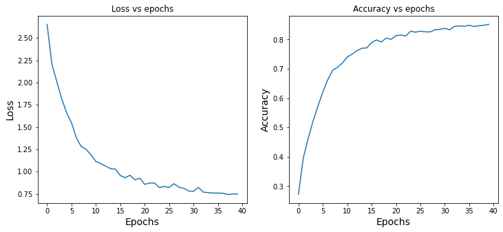
The Residual Network showed better accuracy on the test set, achieving nearly 81% compared to the benchmark model’s 75.6% accuracy. We can easily make the Residual Network deeper to extract more value.
fig, axes = plt.subplots(1, 2, sharex=True, figsize=(12, 5))

axes[0].set_xlabel("Epochs", fontsize=14)
axes[0].set_ylabel("Loss", fontsize=14)
axes[0].set_title('Loss vs epochs')
axes[0].plot(train_loss_results)

axes[1].set_title('Accuracy vs epochs')
axes[1].set_ylabel("Accuracy", fontsize=14)
axes[1].set_xlabel("Epochs", fontsize=14)
axes[1].plot(train_accuracy_results)

plt.show()
Figure 2: Training accuracy and loss evolution of the Residual Network over several epochs:
def test_model(model, test_generator):

    epoch_loss_avg = tf.keras.metrics.Mean()
    epoch_accuracy = tf.keras.metrics.CategoricalAccuracy()

    train_steps_per_epoch = test_generator.n // test_generator.batch_size
    i = 0
    for x, y in test_generator:
        model_output = model(x)
        epoch_loss_avg(loss_obj(y, model_output))
        epoch_accuracy(y, model_output)
        if i>=train_steps_per_epoch:
            break
        i+=1

    print("Test loss: {:.3f}".format(epoch_loss_avg.result().numpy()))
    print("Test accuracy: {:.3%}".format(epoch_accuracy.result().numpy()))

print('ResNet Model')
test_model(resnet_model, validation_generator)
print('Benchmark Model')
test_model(benchmark_model, validation_generator)

ResNet Model
Test loss: 0.787
Test accuracy: 80.945%
Benchmark Model
Test loss: 1.067
Test accuracy: 75.607%

num_test_images = validation_generator.n

random_test_images, random_test_labels = next(validation_generator)

predictions = resnet_model(random_test_images)

fig, axes = plt.subplots(4, 2, figsize=(25, 12))
fig.subplots_adjust(hspace=0.5, wspace=-0.35)

j=0
for i, (prediction, image, label) in enumerate(zip(predictions, random_test_images, target_labels[(tf.argmax(random_test_labels, axis=1).numpy())])):
    if j > 3:
        break
    axes[i, 0].imshow(np.squeeze(image))
    axes[i, 0].get_xaxis().set_visible(False)
    axes[i, 0].get_yaxis().set_visible(False)
    axes[i, 0].text(5., -7., f'Class {label}')
    axes[i, 1].bar(np.arange(len(prediction)), prediction)
    axes[i, 1].set_xticks(np.arange(len(prediction)))
    axes[i, 1].set_xticklabels([l.split('_')[0] for l in target_labels], rotation=0)
    pred_inx = np.argmax(prediction)
    axes[i, 1].set_title(f"Categorical distribution. Model prediction: {target_labels[pred_inx]}")
    j+=1
plt.show()
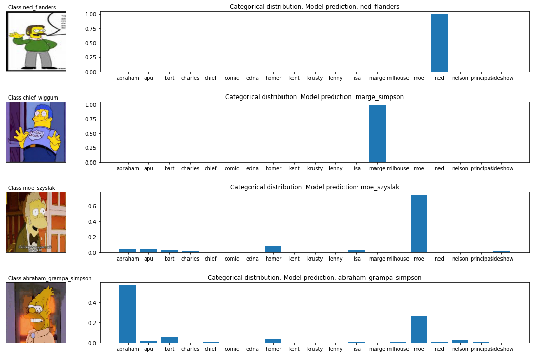
Figure 3: Random images (left) and the corresponding classification distribution generated by the Residual Network (right).
6. Conclusion
The Residual Network has proven capable of stabilizing the optimization process of deep networks. Furthermore, the performance of the Residual Network surpasses that of traditional CNNs, demonstrating the power of shortcut connections.This approach can be scaled by increasing the depth of the model. This is especially applicable in cases where the Residual Network does not have degradation problems.
7. References
[1] [Krizhevsky et al., 2012] Krizhevsky, A., Sutskever, I., and Hinton, G. E. (2012). Imagenet classification with deep convolutional neural networks. Advances in neural information processing systems, 25:1097–1105.[2] [He et al., 2015] He, K., Zhang, X., Ren, S., and Sun, J. (2015). Deep residual learning for image recognition.[3] [He et al., 2016] He, K., Zhang, X., Ren, S., and Sun, J. (2016). Identity mappings in deep residual networks.[4] https://www.kaggle.com/alexattia/the-simpsons-characters-dataset[5] https://towardsdatascience.com/transfer-learning-and-data-augmentation-applied-to-the-simpsons-image-dataset-e292716fbd43
Good news!
Beginner Learning Vision Knowledge Community
Now open to the public👇👇👇
Download 1: OpenCV-Contrib Extension Module Chinese Version Tutorial

Reply "Extension Module Chinese Tutorial" in the background of "Beginner Learning Vision" public account to download the first OpenCV extension module tutorial in Chinese, covering installation of extension modules, SFM algorithms, stereo vision, object tracking, biological vision, super-resolution processing, etc. with more than twenty chapters of content.

Download 2: Python Vision Practical Project 52 Lectures

Reply "Python Vision Practical Project" in the background of "Beginner Learning Vision" public account to download 31 visual practical projects including image segmentation, mask detection, lane detection, vehicle counting, eyeliner addition, license plate recognition, character recognition, emotion detection, text content extraction, and facial recognition, helping to quickly learn computer vision.

Download 3: OpenCV Practical Project 20 Lectures

Reply "OpenCV Practical Project 20 Lectures" in the background of "Beginner Learning Vision" public account to download 20 practical projects based on OpenCV, achieving advanced learning of OpenCV.

Group Chat

Welcome to join the public account reader group to communicate with peers. Currently, there are WeChat groups for SLAM, 3D vision, sensors, autonomous driving, computational photography, detection, segmentation, recognition, medical imaging, GAN, algorithm competitions, etc. (will gradually be subdivided later). Please scan the WeChat ID below to join the group, with the note: "Nickname + School/Company + Research Direction", for example: "Zhang San + Shanghai Jiao Tong University + Vision SLAM". Please follow the format for notes, otherwise, you will not be approved. After successful addition, you will be invited to enter the relevant WeChat group based on your research direction. Please do not send advertisements in the group, otherwise, you will be removed from the group. Thank you for your understanding~