Please click on the four characters “Shanghai Siying” above to follow us. Siying Technology focuses on brain imaging data processing, covering (radiomics,fMRI, structural images, white matter hyperintensity analysis, PVS, PET, spectroscopy, DWI, DTI-ALPS, QSM, ASL, IVIM, DCE, DSC, oxygen extraction fraction (OEF) andCMRO2, BOLD-CVR, primate brain imaging, rodent brain imaging, microbiota, EEG/ERP, magnetoencephalography, FNIRS, eye movement) etc. We hope that professional content can help our followers, and we welcome comments and discussions. We also welcome you to participate in Siying Technology’s courses. You can add WeChat IDsiyingyxf or 18983979082 for inquiries. (Click to browse at the end of the article)
The increasing popularity of machine learning has led to the development of some tools designed to make the application of this method easy for newcomers to machine learning. These efforts have produced tools like PRoNTo and NeuroMiner, which do not require any programming skills. However, while these tools may be very useful, their simplicity comes at the cost of transparency and flexibility. Learning how to program a machine learning pipeline (even a simple one) is a great way to gain insight into the advantages of this analytical method, as well as the distortions that can occur along the machine learning pipeline. Furthermore, it allows for greater flexibility, such as using any machine learning algorithm or data pattern of interest. Despite the obvious benefits of learning how to program a machine learning pipeline, many researchers find it challenging to do so and do not know where to start.
In this article, we provide a step-by-step tutorial on how to implement a standard supervised machine learning pipeline using scikit-learn. scikit-learn is a widely popular and easy-to-use machine learning library in the Python programming language. We provide brief basic principles and explanations of the code at each step of the process, and when relevant, we will provide useful external resources that offer further examples or more in-depth discussions. The example code follows the workflow described in Chapter 2. Readers are encouraged to refer to this chapter for a deeper theoretical explanation of the main elements of the machine learning pipeline.
The target audience for this tutorial is beginners in machine learning. For this reason, it requires minimal programming knowledge. However, readers are encouraged to become familiar with basic Python. Python is a widely used programming language with many available resources. Intermediate users will also find this tutorial useful. The example code is structured in a way that makes it easy to remove, add, or replace certain techniques with others. This way, readers can experiment with different approaches and develop more complex pipelines based on the code. The implementation adheres to a strict methodology to avoid common errors such as double dipping and achieve reliable results. This article is published in Machine Learning Methods and Applications to Brain Disorders. For the original text and supplementary materials, please add the WeChat IDsiyingyxf or 18983979082 for inquiries. Siying also provides a free literature download service. If needed, you can also add this WeChat ID to join the group, and the original text will also be published in the group).
Siying has published multiple articles on the application of machine learning/deep learning in brain imaging. Please read together to deepen your understanding. Thank you for your support.(Click directly to browse.)Add WeChat IDorfor the original text and supplementary materials):
Deep Learning for Brain Age Estimation
Painless Resting-State Functional Connectivity Predicts Individual Pain Sensitivity
Prediction of Suicide Risk in Elderly Depressed Patients Based on Multimodal Brain Connectomics
Brain Age Prediction Using Global-Local Transfer Learning Approaches
Autism Prediction Model Based on Functional Connectomics
AI Diagnosis of Schizophrenia Based on Magnetic Resonance Imaging
JAMA Psychiatry: Clinical, Brain, and Multilevel Clustering in Early Psychosis and Affective Stages
Translational Machine Learning in Child and Adolescent Psychiatry
Application of Deep Learning in Neuroimaging Diagnosis and Rehabilitation of Autism Spectrum Disorders
Exploring the Links Between Mental Illness and Frontotemporal Dementia Using Multimodal Machine Learning Approaches
Heterogeneity Characterization of Neuroimaging, Cognitive, Clinical Symptoms, and Genetics in Elderly Depressed Patients
Machine Learning (HYDRA) Reveals Neuroanatomical Subtypes of Two Schizophrenia Types
Deep Learning for Small Data and Big Data in Psychiatry
Science: Revealing Neuroanatomical Variations in Autism Using Contrastive Machine Learning Approaches
Convolutional Neural Networks
Neuroimaging Predicts Mental Illness and Mental Health Prospects
Multimodal Deep Learning Models for Early Detection of Alzheimer’s Disease Staging
Application of Deep Learning in Resting-State fMRI
Deep Learning Research in Brain Imaging: Prospects and Challenges
Current State and Future Challenges of Explainable AI in MRI-Based Brain Age Studies
A Decade of BrainAGE as a Neuroimaging Biomarker of Brain Aging
Neuroimaging-Driven Brain Age Estimation as a Biological Marker for Identifying Brain Disorders and Health Conditions
Deep Learning Models Based on Raw Imaging Data Predict Reliable Genetic Biomarkers of Brain Age
AJP: Longitudinal Identification Study of Accelerated Brain Aging in Schizophrenia Patients
Deep Learning Models Based on MRI Data Features Predict Brain Age and Disease in a Global Sample of 14,468 Subjects
AJP: Differences in Emotional Circuit Delay Maturation in Abused Girls with and without Internalizing Mental Disorders
Brain Age in Patients with Major Depression
SVM Applications in Brain Imaging Data
Identification of Autism Spectrum Disorder Using Deep Learning and the Autism Brain Imaging Database (ABIDE)
Radiology: Cortical Thickness Predicts Conversion from Mild Cognitive Impairment to Parkinson’s Dementia
Neuroimaging Classification Studies and Relevant Feature Extraction for Alzheimer’s Disease and Its Precursor Staging
Nature Subjournal: Predicting Functional Brain Aging in Familial Alzheimer’s Disease Patients Using Deep Learning
Applications of Machine Learning in Patients with Major Depression: From Classification to Treatment Outcome Prediction
Classification of Schizophrenia Based on Functional MRI Data Using Machine Learning
Enhancing Generalization of Machine Learning Research on Brain-Behavior Relationships Using Multivariate Representational Approaches
Machine Learning Methods for Clinical Psychology and Psychiatry
PLOS Biology: Generalized Brain Network Biomarkers in Major Depression Across Imaging Centers
Nature Medicine: Neuroimaging Biology of Persistent Experimental and Clinical Pain
The Role of Deep Learning in Analyzing MRI of Infant Brains (Part One)
The Impact of Parameter Selection on Aphasia Prediction Models Post-Stroke
If Deep Learning is the Answer, What is the Question?
The Risk of Unexpected Overfitting When Classifying Brain Data
Applications of Machine Learning in Resting-State fMRI
The Role of Supervised Machine Learning in Systems Neuroscience
Nature Protocols: For Explaining Machine Learning Models in Neuroimaging
Biological Psychiatry: Individual Indicators Prediction Based on Multimodal Brain Imaging – Methods
Biological Psychiatry: Advances in Neuro Subtype Research for Autism
PNAS: Gray Matter Age Prediction as a Biomarker for Dementia Risk
BRAIN: Development of an Explainable Deep Learning Framework for Alzheimer’s Disease Classification
Heterogeneity Issues: Methods for Identifying Subtypes of Mental Illness
NPP: Physiological Sex Classification of Structural MRI Data Shows Misclassification of Transgender Women
Classification and Prediction of Brain Disorders Using Functional Connectivity
Prediction of Mental Illness Based on Brain Imaging
Prediction of Treatment Outcomes for Chronic Pain Based on Imaging and Quantitative Sensory Testing
Identifying Optimal Data-Driven Feature Selection Methods to Improve Reproducibility in Classification Tasks
Neuron Brain Imaging Machine Learning: Characterization, Pattern Information, and Brain Features
Molecular Psychiatry: Resting-State fMRI Predicts Cognitive Abilities in Adolescents
JAMA Psychiatry: Brain Imaging Machine Learning Predicts Social Functioning in Patients with Mental Illness
AJP: Cocaine Withdrawal Prediction Based on Brain Networks
Diagnosis of Mood Disorders Based on Machine Learning: Functional Networks Predict Drug Response
Brain Imaging Features Predict Onset Timing of Sporadic Alzheimer’s Disease Symptoms
We will first briefly introduce how to install Python and all necessary libraries, as well as how to access the dataset and online version of the code.
19.2 InstallingPython and Major Libraries
In this tutorial, the source code is written in Python 3. Like most programming languages, Python is organized in libraries. Each library contains a set of dedicated functions for specific purposes. In this tutorial, we use the following libraries:
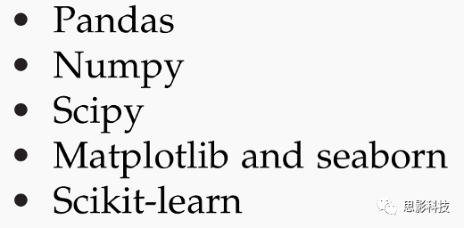
Pandas and numpy are widely used libraries for loading, manipulating, and summarizing data. While pandas is used for handling tabular data (for example, data arranged in tables with rows and columns), numpy is a more general-purpose library. We also use the foundational library for scientific computing, scipy, to run some univariate statistics to explore the data and prepare for statistical analysis. Matplotlib and seaborn are libraries for data visualization, which is very useful when researching data or summarizing results. Finally, scikit-learn, or more commonly known as sklearn, is arguably the most popular and accessible machine learning Python library. It is a high-level library, meaning that many complex applications are encapsulated in simpler, shorter, and easier-to-use functions.
To run the example code in this tutorial, readers need to install Python 3 and all the libraries mentioned above. The easiest way is to download and install Anaconda. This is a free and open-source distribution of the Python programming language designed for scientific computing, aimed at simplifying package management and deployment.
19.3 How to Read This Chapter
In this chapter, readers will find different text styles distinguishing different types of information. Code blocks (called code snippets) will appear in boxes below. Code snippets are numbered for easier reference to the different stages of the analysis. The output of each code snippet is displayed below the code.

In some cases, a line of code may be too long and must be split into two lines. This will be indicated by \ (note that this is not in the online version of the code). The online version of the example code is written in notebook format. >>> indicates that the output of the command will be displayed in the notebook. For some code snippets, the output may be too long, in which case only part of the output will be shown. This will be marked as “… .” References to major libraries or specific tools in particular libraries are displayed in courier new font.
19.4 Using Brain Morphometry to Classify Schizophrenia Patients and Healthy Controls
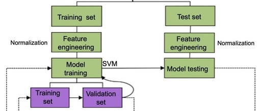
The example used in this tutorial involves using neuroanatomical data to classify schizophrenia patients (SZ) and healthy controls (HC).The simulated FreeSurfer output dataset contains gray matter volumes and thicknesses of 101 brain regions, as well as each participant’s ID, age, sex, and diagnosis. Figure 19.1 illustrates an overview of the final workflow implemented in this tutorial. For the purpose of this exercise, we assume that feature extraction, i.e., the process of extracting volume and thickness values from raw structural magnetic resonance imaging (MRI) images, has already been completed. Thus, we start our tutorial by preparing the data for machine learning analysis. In this step, we will explore missing data, confounding variables, and class imbalance data, and discuss how to address these issues. Next, we define a cross-validation (CV) scheme with 10 iterations (external CV). In each iteration, the training and testing sets undergo data transformations separately to avoid knowledge leakage. Then, a support vector machine (SVM) model is used for the training set.SVM relies on a hyperparameter C. To decide which value of C to use, we create an internal 10-fold CV. This means that for each C value we want to test, an SVM model will be trained and tested 10 times; for a given C value, the final performance is estimated by averaging the performance of the 10 runs. The SVM model is then trained on the entire training set using the optimal C parameter. The performance of the trained model is measured in the testing set. The entire process is repeated 10 times (i.e., 10 iterations of external CV). Once completed, the final performance of our SVM model is calculated by averaging the performance metrics from the 10 external folds. Finally, we investigate which features are more important in driving the model’s predictions and test the statistical significance of the final performance of our model.
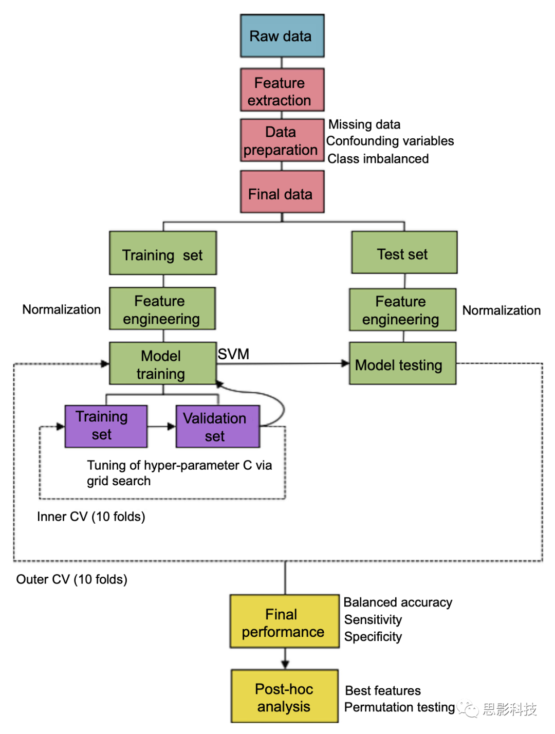
Figure 19.1 Overview of the machine learning workflow implemented in this tutorial.
The machine learning pipeline used in our example includes the following components:Problem formulation, data preparation, feature engineering, model training, model evaluation, and post-analysis. Before we begin, we first need to import all necessary libraries, set a fixed random seed, and organize our workspace.
19.5.1Importing Libraries
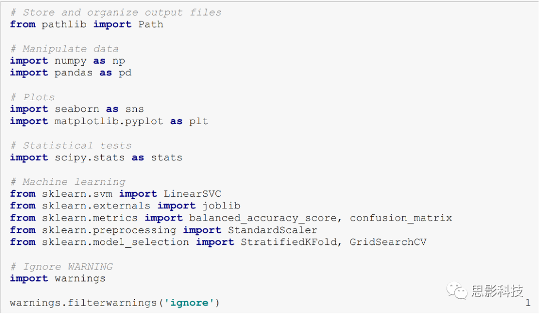
By default, libraries for performing machine learning analysis are not loaded. Therefore, it is best practice to import all the libraries we need at the beginning of the code file. In addition to pandas, numpy, scipy, seaborn, matplotlib, and sklearn, we also use the pathlib module to organize folders and the warnings module to suppress any unnecessary warnings during the analysis (both are built into Python, so we do not need to install them). If readers decide to modify the code, we recommend reactivating warnings by suppressing the last line in code snippet 1. Understanding these warnings can help readers avoid errors and debug the code. To make the code easier to read, it is common to specify an alias when importing frequently used libraries. For example, the pandas library is often imported as pd. This way, whenever we want to call this library, we just need to type pd.
19.5.2 Setting a Random Seed
Some steps in our analysis will be influenced by randomness. For example, we may want to randomly remove some participants during data cleaning. Similarly, when defining the CV scheme, the training/testing partition for each iteration is also done randomly. In Python, this randomness can be controlled by setting the seed value to a fixed number. Not defining a specific seed value means that variables relying on this element of randomness will behave differently each time we run the code. For example, the training/testing partition for each iteration will be different, which may lead to varying model performance. Therefore, we set the seed value to a fixed number to ensure that we obtain the same results each time we run the code. Some functions require passing the random seed as a parameter again.

19.5.3 Organizing the Workspace
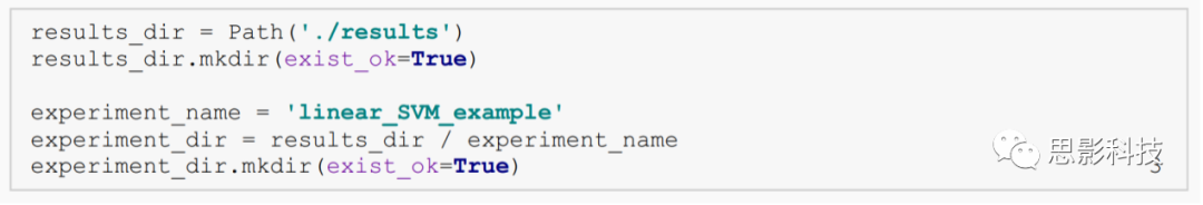
Before starting the analysis, we should first create a folder structure to store all results. In this tutorial, readers may want to test different strategies along the machine learning pipeline, such as different preprocessing strategies or machine learning algorithms. After extensive testing, it is easy to forget which results correspond to which strategies. It is a good practice to assign a name to each experiment, create a folder with the same name in the results directory, and store the experimental outputs in that directory.
19.5.4 Problem Formulation
When undertaking any type of project, having a good framework for the problem is crucial, especially in machine learning, where there may be many possible ways to analyze the same dataset. In this tutorial, our machine learning problem is as follows:
Classifying SZ and HC patients using structural MRI data.
From this formulation, we can derive the main elements of the machine learning problem:

The purpose of this step is to perform a series of statistical analyses to prepare the data for the machine learning model. Here, depending on the nature of the machine learning problem and the type of data, different statistical analyses may be required.
In this tutorial, we use tabular data. The data is stored in the form of a comma-separated values (CSV) file. We use the read_csv() function from pandas to load the csv file. This function loads the data into an object type called dataframe, which we name dataset_df.

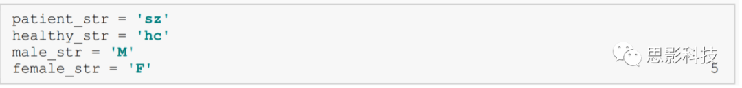
In our dataset, diagnosis and sex are defined by words. Sometimes, people store information using different names; for example, in the diagnosis column, instead of using sz, we can define this problem as belonging to a patient using the word “schizophrenia”. To make these codes more adaptable to different formats, we defined our symbols at the beginning of the code.
Let’s start by looking at the first six rows of the data. Selecting a subset of a dataframe is straightforward using pandas. There are different ways to do this. Here, we simply point out the indices we need in the dataframe (note that the first row index is 0 and the last row is not included).
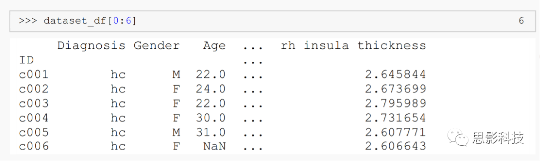
From the output, we can see the column names at the top and the data for the first six participants. The columns include diagnosis, sex, age, and gray matter volumes and thicknesses of several brain regions.ID is set as the column index in code snippet 4. We can see that at least one value is missing (row c006). We will address this issue later.
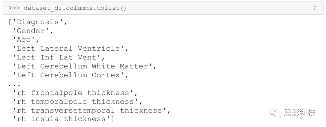
It may also be useful to know the names of all the features available in the dataset. For this, we just need to know the names of the data columns.
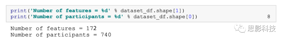
Next, check the size of the dataset.
 To address some of the most common issues when building a machine learning pipeline, our data preparation phase will check the following datasets:

Most machine learning models do not support data with missing values. Therefore, it is important to check if there are any missing values in dataset_df. Below, we use the function isnull() from pandas to determine how much missing data there is for each feature and the ID of the participants with missing data.
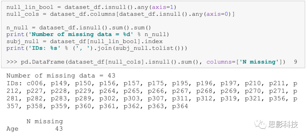
We can see that there are 43 missing age values. Without this information, a thorough assessment of the unbalanced population data cannot be conducted, which may pose problems when interpreting the results. There are many different options of varying complexity for handling this (more information on these options can be found in Chapter 14).Because deleting these participants would only lose 6% of the total data, we will simply remove them. We can do this by using the dropna() function from pandas.
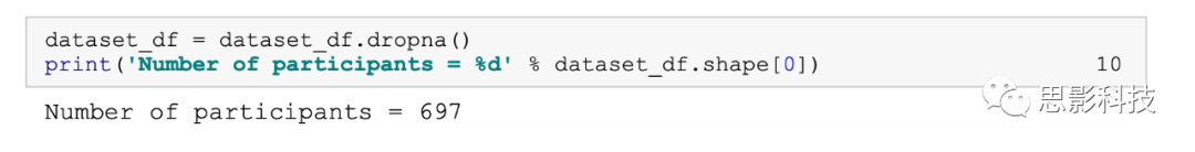
As expected, the new dataframe is now 43 participants less than before.
Next, let’s check the total number of individuals in each class:
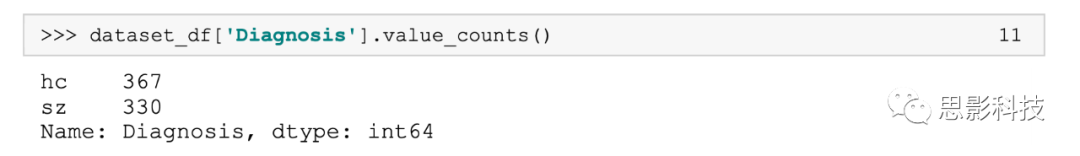
In our dataset, there are 367 controls and 330 patients. There does not seem to be a significant imbalance between the classes. However, the two classes do not match perfectly. As mentioned in Chapter 2, this may pose issues when estimating model performance. One option is to downsample the HC group to match the SZ group. However, this would mean losing more data in addition to the 6% we have already discarded, which is undesirable. Since the imbalance is not too great, we will retain the same data and use balanced accuracy as our chosen performance metric, along with a stratified CV scheme to ensure that the ratio of SZ/HC remains the same in the CV iterations.
19.5.5.4 Confounding Variables
One may want to examine many potential confounding variables. Here, we will investigate two obvious issues: sex and age.
One simple way to examine sex as a potential confounding factor is to verify the ratio of males and females in the patient and control groups. Let’s first visualize the sex ratio in each group using seaborn. Using this library to plot the data is very simple (https://seaborn.pydata.org). Note that seaborn operates based on another library called matplotlib, which is the most widely used plotting library in Python.
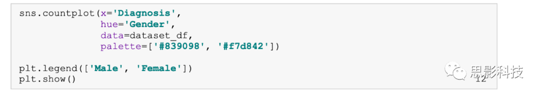
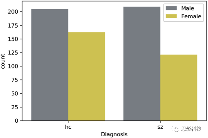
We can see that the number of males in the two groups is quite similar. However, the control group has more females than the patient group. Besides visualizing the data, it is always best practice to perform appropriate statistical tests even when there are no apparent biases in visual inspection. Since sex is a categorical variable, we will use a chi-square test for homogeneity to examine whether this difference is statistically significant. In this case, we want to test the null hypothesis that the proportion of females in the HC group is not different from the proportion of females in the patient group(equivalent to testing that the proportion of males in the HC group is not different from the proportion of males in the patient group).
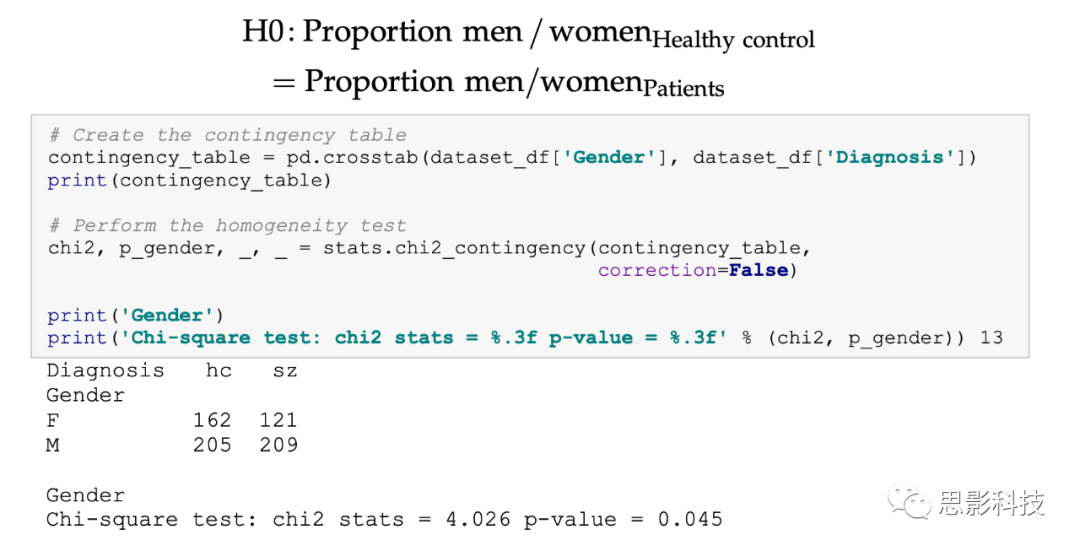
The results above indicate that there is indeed a statistically significant difference between the two categories in terms of sex (p<.05).
This could be a problem, as the impact of sex on brain morphology is well-recognized. Therefore, the machine learning algorithm may use brain features related to sex differences to distinguish HC and SZ, rather than differences related to the disorder being studied.
To mitigate this potential source of bias, we will iteratively randomly remove one female from the HC class until the ratio of males to females between the two classes is no longer statistically significant.
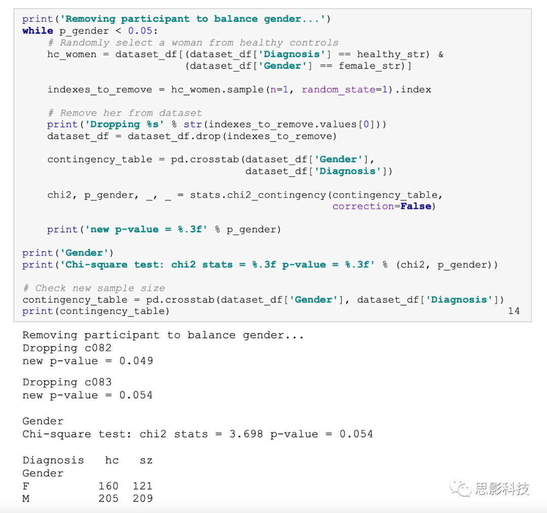
From the output, we can see that after removing two females from the control group, the chi-square test is no longer statistically significant.
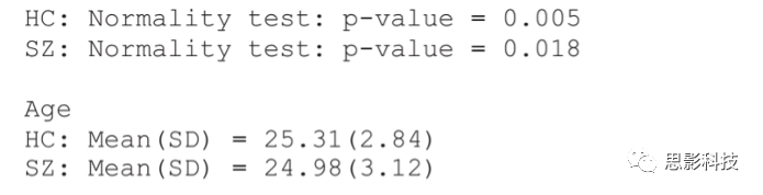
Next, let’s check the imbalance related to age.The idea is to test the null hypothesis that the mean age (or median) of the HC group is not different from the mean age (or median) of the SZ group. One way to do this is to use a parametric t test for the two samples. It is important to note that this test assumes that age is normally distributed in both groups (Gaussian distribution). To check this assumption, we can use the shapiro Wilk test from the scipy library along with seaborn to plot the distribution for each group.
From the above, we can see that age is normally distributed in both groups. Furthermore, the distributions, means, and standard deviations between the two groups are also quite similar. This means we can use t tests to check for statistical differences in age between the groups.

It can be seen that there is no statistically significant age difference between the two groups. Therefore, in our analysis, we will not consider age to be an important confounding factor.
19.5.5.5Feature Set and Target
Our next step is to retrieve the target and features from dataset. For the target variable, we will assign the diagnosis column in dataset_df to the variable targets_df. For these features, we select all rows starting from the fourth column (Recall that the index of dataframes is 0) and save them in features_df.

The cleaned dataset contains 695 subjects and 169 features. This number of subjects is much higher than the recommended sample size of 130 to obtain stable results. However, in many studies on brain disorders, our sample size may be smaller. In these cases, caution must be exercised, as a sample size smaller than the optimal size may lead to unreliable results.
Next, let’s save the cleaned data into a CSV file in the created directory.

19.5.6 Feature Engineering
In this step, we want to perform a series of transformations on our data that will help us build a good machine learning model. As discussed in Chapter 2, this series of transformations may involve different processes depending on the nature of the data. Below, we will discuss each step in the same order as in Chapter 2.
19.5.6.1 Feature Extraction
In our example, we want to classify SZ and HC using neuroanatomical data. This requires extracting brain morphological feature information from raw MRI images. As mentioned earlier, in this tutorial, we assume that this feature extraction has already been completed for us.The gray matter volumes and thicknesses that make up the features_df variable have already been extracted by FreeSurfer.
19.5.6.2 Cross-Validation (CV)
Before applying any transformations to our features, we first need to split the data into training and testing sets. Recall that this is a key step to ensure independence between the training and testing steps of the machine learning analysis. In this tutorial, we use stratified 10-fold CV. Chapter 2 outlines some of the most commonly used types of CV.
First, we transform targets_df into a 1D numpy array where 0 represents HC and 1 represents SZ; we will call this new variable targets. By transforming targets_df into a 2D numpy array, we perform the same process on the features. Transforming data from dataframes to arrays will make it easier, as some functions require data in this format.

Next, we define the parameters for stratified 10-fold CV by creating an object from the StratifiedKFold class in the sklearn library. We will call this object skf.

Note the parameter random_state in skf. This parameter allows us to control the inherent randomness element that divides the entire dataset into training and testing sets. Our dataset contains a total of 695 participants. In the code above, we have instructed the model to divide the dataset into 10 groups (while maintaining the ratio of SZ/HC similar throughout the CV iterations). In these cases, Python will perform this grouping randomly. Not setting the random state to a fixed value means that the participants assigned to each group will be different each time we run the code. Therefore, our results are likely to vary as well. This is something we want to avoid, at least while we are building the model to improve it, as we want to be able to reproduce the same results when comparing different models.
Next, we prepare a set of empty objects that will be filled with predictions, performance metrics, and the coefficients of the machine learning model for each iteration of the CV. In the code below, we create:
(1) an empty dataframe called predictions_df that will store the model’s predictions;
(2) three empty arrays for each performance metric: balanced accuracy(bac), sensitivity(sens), specificity(spec);
(3) An empty array of coefficients for the SVM, where the weight (coefficient or importance) of each feature will be stored. Finally, we also create an additional folder called model dir, which will later save all the above objects.

Now that we have defined the CV, we can iterate through each of the 10 iterations of CV. In each iteration, we will perform any transformations (e.g., feature selection, normalization) on the training set, and fit the machine learning algorithm to the same data; then, we will use the testing set to test the algorithm after applying the same data transformations that were applied to the training set. This can be achieved using a for loop to iterate through the 10 i_folds. In each i_folds, we will have four new variables:
(1) features_train and targets_train : the training set and corresponding labels;
(2) features_test and targets_test: the testing set and corresponding labels;
Now, let’s check how many participants are in the training and testing sets during each iteration of CV. We can do this by simply setting the lengths of targets_train and targets_test.

Note how the code inside the for loop is indented further to the right. This is called indentation, which means that the instructions in the indented code block will be executed in each iteration of CV. The next code segments (22 to 31) will maintain the same indentation, indicating that they are still part of this for loop. Once the CV is completed, the indentation will be removed, meaning that the text will be placed again from the left edge of the text box. Note that if you run this code, all loop segments will need to run together. Also, note that the folds are numbered starting from 0, not 1; this is because in Python, the for loop index is 0.
19.5.6.3 Feature Selection
As discussed in Chapter 2, feature selection can help us remove redundancy from the feature set. However, given that the neuroanatomical abnormalities of SZ are often subtle and widespread, we have reason to assume that most of the 169 features in our feature set will contribute to distinguishing between patients and controls. Additionally, we note that in our example, the number of features is not too large compared to the total sample size. For these reasons, we will not remove features. If we were to use feature selection, there would be a lot of strategies available through sklearn.
19.5.6.4 Feature Normalization
Before feeding the data into the classifier, we want to ensure that the situation where measurements from different brain regions have different measurement ranges does not affect the reliability of our model. If the variance of one feature is several orders of magnitude larger than that of other features, then that feature may dominate the other features in the dataset.
There are several possible solutions to avoid this issue. In this example, we will transform the data so that the distribution of each feature is similar to a standard normal distribution (e.g., mean 0 and variance 1). Each new normalized value Zxi is obtained by taking each data point xi, subtracting the corresponding feature’s mean X, and then dividing by the standard deviation (SD) of the same feature:

We can use the StandardScaler object in sklearn to automatically apply this formula independently to each feature.

First, we create a scaler object. Then, we fit the scaler parameters (mean and standard deviation) to the training set. In other words, we calculate and store the mean X and SD of each feature in the training set in the scaler object. Then, we transform both the training and testing sets using the stored parameters with the formula above. Sklearn also provides other extended strategies; for example, if the distribution is not normal or there are several outliers, the function RobustScaler() would be more suitable.
If you are interested in brain imaging and machine learning data processing, you can participate in relevant courses offered by Siying Technology. For details, please browse the following links(You can add WeChat IDsiyingyxf or 18983979082 for inquiries. Siying also provides a free literature download service. If needed, you can also add this WeChat ID to join the group):
38th Magnetic Resonance Brain Network Data Processing Class (Nanjing, 6.7-12)
29th Brain Imaging Machine Learning Class (Nanjing, 6.15-20)
86th Magnetic Resonance Brain Imaging Basic Class (Nanjing, 7.6-11)
12th Magnetic Resonance ASL Data Processing Class (Nanjing, 7.14-17)
83rd Magnetic Resonance Brain Imaging Basic Class (Chongqing, 6.9-14)
13th Brain Network Data Processing Advanced Class (Chongqing, 7.3-8)
27th Magnetic Resonance Brain Imaging Structural Class (Chongqing, 7.15-20)
87th Magnetic Resonance Brain Imaging Basic Class (Chongqing, 7.23-28)
Beijing:
10th Radiomics Class (Updated: Beijing, 6.11-16)
39th Magnetic Resonance Brain Network Data Processing Class (Beijing, 6.20-25)
84th Magnetic Resonance Brain Imaging Basic Class (Beijing, 6.28-7.3)
8th Diffusion Magnetic Resonance Imaging Advanced Class (Beijing, 7.18-23)
33rd Diffusion Imaging Data Processing Class (Shanghai, 6.22-27)
85th Magnetic Resonance Brain Imaging Basic Class (Shanghai, 6.28-7.3)
11th Radiomics Class (Shanghai, 7.12-17)
15th Task-Based Functional Magnetic Resonance Data Processing Class (Shanghai, 7.19-24)
Data Processing Business Introduction:
Siying Technology Functional Magnetic Resonance (fMRI) Data Processing Business
Siying Technology Diffusion Weighted Imaging (DWI) Data Processing
Siying Technology Brain Structural Magnetic Resonance (T1) Imaging Data Processing Business
Siying Technology Rodent (Rat and Mouse) Neuroimaging Data Processing Business
Siying Technology Quantitative Susceptibility Mapping (QSM) Data Processing Business
Siying Technology Radiomics Data Processing Business
Siying Technology DTI-ALPS Data Processing Business
Siying Data ASL Data Processing Business
Siying Technology Primate fMRI Analysis Business
Siying Technology Brain Imaging Machine Learning Data Processing Business Introduction
Siying Technology Microbiota Analysis Business
Siying Technology EEG/ERP Data Processing Business
Siying Technology Near-Infrared Brain Function Data Processing Service
Siying Technology EEG Machine Learning Data Processing Business
Siying Data Processing Service Six: Magnetoencephalography (MEG) Data Processing
Siying Technology Eye Movement Data Processing Service
Recruitment and Products:
Siying Technology is recruiting Data Processing Engineers (Beijing, Shanghai, Nanjing, Chongqing)
BIOSEMI EEG System Introduction
Eyepiece Functional Magnetic Resonance Stimulation System Introduction
Here, give a “Like” and “Share” to let more friends pay attention