Research on Intelligent Quantitative Trading System Based on Deep Hybrid Architecture

Source: DeepHub IMBA

This article is approximately 5500 words, recommended reading time is over 10 minutes.
This article explores the hybrid modeling method that combines temporal features and static features in the field of quantitative trading.

By integrating Stacked Sparse Denoising Autoencoder (SSDA) and Long Short-Term Memory based Autoencoder (LSTM-AE), we aim to build a trading system that can comprehensively capture the dynamic characteristics of the market.

Feature Representation Learning

During the feature engineering phase, SSDA extracts robust representations of stock data through denoising techniques. This method effectively filters out market noise while retaining key features that have a substantial impact on price trends, such as trend change points and abnormal fluctuations.

 import numpy as np
import pandas as pd
from sklearn.preprocessing import MinMaxScaler
from tensorflow.keras.models import Model
from tensorflow.keras.layers import Input, Dense, Dropout
from tensorflow.keras.optimizers import Adam
import tensorflow as tf

mse_loss = tf.keras.losses.MeanSquaredError()

# SSDA model construction function
def build_ssda(input_dim):
    """
    Build a Stacked Sparse Denoising Autoencoder (SSDA) model.
        Parameters:
    - input_dim: Input feature dimension (corresponding to the length of the stock data time window).
        Returns:
    - ssda: Compiled Keras model.
    """
    input_layer = Input(shape=(input_dim,))
    encoded = Dense(16, activation='relu')(input_layer)  # Encoding layer
    encoded = Dropout(0.1)(encoded)  # Introduce Dropout for regularization
    decoded = Dense(input_dim, activation='linear')(encoded)  # Decoding reconstruction layer

    ssda = Model(inputs=input_layer, outputs=decoded)
    ssda.compile(optimizer=Adam(learning_rate=0.001), loss='mse')
    return ssda

# Data preprocessing: Extract and normalize adjusted closing prices
prices = data['Adj Close'].values.reshape(-1, 1)
scaler = MinMaxScaler()
normalized_prices = scaler.fit_transform(prices).flatten()

# Define sliding window parameters
window_size = 20

# Build training dataset
ssda_train_data = np.array([
    normalized_prices[i:i + window_size]
    for i in range(len(normalized_prices) - window_size)
])

# Build and train SSDA model
ssda = build_ssda(input_dim=window_size)

# Model training
ssda.fit(
    ssda_train_data,
    ssda_train_data,  # The goal of the autoencoder is to reconstruct the input data
    epochs=50,
    batch_size=32,
    shuffle=True,
    verbose=1
)

# Model persistence
ssda.save("ssda_model.h5")
print("SSDA model saved as 'ssda_model.h5'.")

Temporal Pattern Modeling

The LSTM autoencoder focuses on capturing the temporal dependencies of the market. By modeling the price sequence within a sliding window, the system can learn the periodic characteristics and long-term dependencies of the market, thus better understanding the historical context and future trends of price changes.

 from tensorflow.keras.layers import Input, LSTM, RepeatVector
from tensorflow.keras.models import Model
import tensorflow as tf

# Define loss function
mse_loss = tf.keras.losses.MeanSquaredError()

def build_lstm_ae(timesteps, input_dim):
    """
    Build LSTM autoencoder model.
        Parameters:
    - timesteps: Length of the time series.
    - input_dim: Feature dimension at each time step.
        Returns:
    - lstm_ae: LSTM autoencoder model.
    """
    # Define input layer
    inputs = Input(shape=(timesteps, input_dim))
    # Encoder part
    encoded = LSTM(16, activation='relu', return_sequences=False)(inputs)
    # Decoder part
    decoded = RepeatVector(timesteps)(encoded)
    decoded = LSTM(input_dim, activation='linear', return_sequences=True)(decoded)
    # Build complete model
    lstm_ae = Model(inputs, decoded)
    lstm_ae.compile(optimizer='adam', loss='mse')
    return lstm_ae

# Set model hyperparameters
timesteps = 20  # Time window length
input_dim = 1   # Univariate input (adjusted closing price)
# Build and train LSTM autoencoder
lstm_ae = build_lstm_ae(timesteps, input_dim)
features = data['Adj Close'].values.reshape(-1, 1)
lstm_train_data = np.array([features[i:i + timesteps] for i in range(len(features) - timesteps)])
lstm_ae.fit(lstm_train_data, lstm_train_data, epochs=100, batch_size=32, shuffle=True)

State Augmentation Mechanism

This article proposes a state augmentation mechanism, which constructs an enhanced state space that integrates the outputs of SSDA and LSTM-AE, representing both static features and dynamic temporal dependencies. This enhanced state will serve as the decision basis for the reinforcement learning agent.

 import numpy as np

t = 20  # Ensure time step is not less than window size
window_size = 20

def get_augmented_state(adj_close_prices, t, window_size, ssda, lstm_ae):
    """
    Generate augmented state representation based on SSDA and LSTM-AE models.
        Parameters:
    - adj_close_prices: Adjusted closing price series.
    - t: Current time step.
    - window_size: Feature extraction window size.
    - ssda: Pre-trained SSDA feature extractor.
    - lstm_ae: Pre-trained LSTM-AE sequence encoder.
        Returns:
    - augmented_state: Combined feature vector.
    """
    # Validate time step validity
    if t < window_size - 1:
        raise ValueError(f"Invalid slicing at t={t}. Ensure t >= window_size - 1.")
    # Extract numerical features
    features = adj_close_prices.iloc[t - window_size + 1:t + 1].values.reshape(-1, 1)
    # SSDA feature extraction
    ssda_features = ssda.predict(features.reshape(1, -1)).flatten()
    # LSTM-AE sequence encoding
    lstm_input = features.reshape(1, window_size, 1)
    lstm_features = lstm_ae.predict(lstm_input).flatten()
    # Feature fusion
    augmented_state = np.concatenate((ssda_features, lstm_features))
    # Dimension normalization
    if len(augmented_state) < window_size:
        # Zero padding when features are insufficient
        augmented_state = np.pad(augmented_state, (0, window_size - len(augmented_state)), mode='constant')
    elif len(augmented_state) > window_size:
        # Truncate when features are excessive
        augmented_state = augmented_state[:window_size]
    return augmented_state
    # Generate augmented state example
augmented_state = get_augmented_state(adj_close_prices, t, window_size, ssda, lstm_ae)
print("Augmented State:", augmented_state)

Reinforcement Learning Framework Design

This article adopts the Advantage Actor-Critic (A2C) algorithm as the core of the reinforcement learning framework. The A2C algorithm achieves efficient decision learning in complex financial market environments through the collaborative action of the actor network and the critic network.

Framework Composition

1. Actor Network

• Responsible for generating the probability distribution of trading actions (buy, sell, hold)
• The optimization goal is to maximize expected returns

• Evaluates the value function of the current state
• Provides action evaluation feedback to the actor network

• Integrates the outputs of the actor and critic

• Used to evaluate the degree of advantage of actions relative to average performance

This architecture design fully considers the particularities of the financial market, allowing the actor network to explore potential profit opportunities while ensuring the stability and reliability of strategies through the value assessment of the critic network. This balance mechanism of exploration and exploitation makes the system particularly suitable for handling highly complex and dynamically changing environments like the stock market.

 import numpy as np
class A2CAgent:
    def __init__(self, state_size, action_size, gamma=0.99, alpha=0.001, beta=0.005, initial_balance=1000, epsilon=0.1):
        self.state_size = state_size
        self.action_size = action_size
        self.gamma = gamma  # Discount factor
        self.alpha = alpha  # Actor learning rate
        self.beta = beta    # Critic learning rate
        self.balance = initial_balance
        self.inventory = []
        self.epsilon = epsilon  # Exploration rate
        self.actor_model = self.build_actor()
        self.critic_model = self.build_critic()

    def build_actor(self):
        model = tf.keras.Sequential([
            Dense(32, input_shape=(self.state_size,), activation='relu'),
            Dense(16, activation='relu'),
            Dense(self.action_size, activation='softmax')
        ])
        model.compile(optimizer=Adam(learning_rate=self.alpha), loss='categorical_crossentropy')
        return model

    def build_critic(self):
        model = tf.keras.Sequential([
            Dense(32, input_shape=(self.state_size,), activation='relu'),
            Dense(16, activation='relu'),
            Dense(1, activation='linear')
        ])
        model.compile(optimizer=Adam(learning_rate=self.beta), loss='mse')
        return model

    def get_action(self, state):
        if np.random.rand() < self.epsilon:  # Exploratory decision
            return np.random.choice(self.action_size)
        else:  # Exploitative decision
            policy = self.actor_model.predict(state.reshape(1, -1), verbose=0)[0]
            temperature = 1.0  # Policy temperature parameter
            policy = np.exp(policy / temperature) / np.sum(np.exp(policy / temperature))
            return np.random.choice(self.action_size, p=policy)

    def train(self, state, action, reward, next_state, done):
        value = self.critic_model.predict(state.reshape(1, -1), verbose=0)
        next_value = self.critic_model.predict(next_state.reshape(1, -1), verbose=0)
        advantage = reward + self.gamma * (1 - int(done)) * next_value - value
        # Advantage function normalization
        advantage = (advantage - np.mean(advantage)) / (np.std(advantage) + 1e-8)
        # Action encoding
        actions = np.zeros([1, self.action_size])
        actions[0, action] = 1.0
        # Model update
        self.actor_model.fit(state.reshape(1, -1), actions, sample_weight=advantage.flatten(), verbose=0)
        self.critic_model.fit(state.reshape(1, -1), value + advantage, verbose=0)

Risk-Return Modeling

We adopt a multidimensional reward calculation mechanism that comprehensively considers factors such as trading profitability, market volatility, and maximum drawdown. This design philosophy is consistent with modern portfolio theory, aiming to maximize returns at an acceptable risk level. The design of the advantage function ensures that the system can effectively control risk exposure while pursuing high returns.

 def compute_reward(profit, volatility, drawdown, risk_penalty=0.1, scale=True, volatility_threshold=0.02, drawdown_threshold=0.05):
    """
    Multidimensional reward calculation function.
        Parameters:
    - profit: Trading profit.
    - volatility: Market volatility.
    - drawdown: Maximum drawdown ratio.
    - risk_penalty: Risk penalty coefficient.
    - scale: Whether to normalize the input.
    - volatility_threshold: Volatility threshold.
    - drawdown_threshold: Drawdown threshold.
        Returns:
    - reward: Comprehensive reward value.
    """
    # Input normalization processing
    if scale:
        volatility = min(volatility / volatility_threshold, 1.0)
        drawdown = min(drawdown / drawdown_threshold, 1.0)
    # Calculate comprehensive reward
    reward = profit - risk_penalty * (volatility + drawdown)
    return reward

Overall System Architecture

Data Processing and State Representation

First, the original market data is preprocessed, and feature sequences are constructed using the sliding window method. These data are then subjected to feature extraction and dimensionality reduction through SSDA and LSTM-AE, ultimately generating an augmented state representation that includes both market static features and dynamic features.

A2C Decision Mechanism

Based on the augmented state representation, the actor network outputs the probability distribution of trading decisions, while the critic network evaluates the value of the current market state. This dual-network collaborative mechanism can ensure decision stability while maintaining the ability to explore new trading opportunities.

Evaluation and Feedback System

After executing trades, the system evaluates trading performance through a comprehensive reward function and uses the evaluation results to update the parameters of the actor and critic networks, continuously optimizing trading strategies.

System Implementation and Training Process

The training process adopts a multi-iteration approach, where the agent needs to make a series of trading decisions in the current market environment during each training round. The system guides the agent to form robust trading strategies through a well-designed reward and punishment mechanism: buying operations are set with a small penalty to avoid over-investment, selling operations are rewarded based on price increases, and holding operations are set with slight penalties to prevent excessive conservatism.

 import gc
from tqdm import tqdm

# Training parameter configuration
window_size = 20
episode_count = 15  # Number of training rounds
batch_size = 32

# Initialize trading agent
agent = A2CAgent(state_size=window_size, action_size=3, initial_balance=1000)

# Training main loop
for e in tqdm(range(episode_count), desc="Training Episodes", unit="episode"):
    print(f"\n--- Episode {e+1}/{episode_count} ---")
    # Initialize training state
    start_t = window_size - 1
    state = get_augmented_state(adj_close_prices, start_t, window_size, ssda, lstm_ae)
    total_profit = 0
    agent.inventory = []  # Clear trading positions
    # Single round training process
    for t in range(start_t, len(data) - 1):
        # Get market data
        current_price = data['Adj Close'].iloc[t]
        next_price = data['Adj Close'].iloc[t + 1]
        # Agent decision
        action = agent.get_action(state.reshape(1, -1))
        next_state = get_augmented_state(adj_close_prices, t + 1, window_size, ssda, lstm_ae)
        # Initialize reward calculation
        reward = 0
        done = t == len(data) - 2
        # Trade execution and reward calculation
        if action == 0:  # Buy decision
            if len(agent.inventory) < 100:  # Position control
                agent.inventory.append(current_price)
                print(f"Buy: {current_price:.2f} at time {t}")
                reward = -0.01  # Buying risk penalty
        elif action == 2 and agent.inventory:  # Sell decision
            bought_price = agent.inventory.pop(0)  # Get the purchase price
            profit = current_price - bought_price
            reward = max(profit, 0)  # Positive profit reward
            total_profit += profit
            print(f"Sell: {current_price:.2f} at time {t} | Profit: {profit:.2f}")
        else:  # Hold decision
            print(f"Hold: No action at time {t}")
            reward = -0.005  # Holding cost penalty
        # Strategy update
        agent.train(
            state.reshape(1, -1),
            action,
            reward,
            next_state.reshape(1, -1),
            done=done
        )
        state = next_state
    # Training round summary
    print(f"Episode {e+1} Ended | Total Profit: {total_profit:.2f}")
    # Model persistence
    if e % 5 == 0:
        agent.actor_model.save(f"actor_model1_ep{e}.h5")
        agent.critic_model.save(f"critic_model1_ep{e}.h5")
    # Memory management
    gc.collect()

Experimental Evaluation and Result Analysis

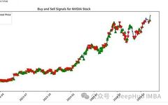
We selected three stocks with varying volatility characteristics for testing: Tesla (medium volatility), Amazon, and NVIDIA. During the testing process, the system needs to make trading decisions based on actual market data and evaluate system performance through cumulative returns. Meanwhile, we recorded buy and sell signals and visually analyzed the system’s decision-making patterns.

 import matplotlib.pyplot as plt
import pandas as pd
import yfinance as yf

# Data acquisition and preprocessing
data = yf.download('AMZN', start='2024-01-01', end='2024-11-01')
data.columns = data.columns.droplevel(1)
data = data.reset_index()
data['Date'] = pd.to_datetime(data['Date'])
print("Available columns:", data.columns)

adj_close_prices = data.get("Adj Close", data["Close"])
print(adj_close_prices.head())

def evaluate_agent(agent, adj_close_prices, window_size, ssda, lstm_ae):
    """
    Trading agent evaluation function
    """
    state = get_augmented_state(adj_close_prices, window_size, window_size, ssda, lstm_ae)
    total_profit = 0
    buy_signals = []
    sell_signals = []
    profits = []
    agent.inventory = []
    # Evaluation loop
    for t in range(window_size, len(adj_close_prices) - 1):
        action = agent.get_action(state.reshape(1, -1))
        next_state = get_augmented_state(adj_close_prices, t + 1, window_size, ssda, lstm_ae)
        current_price = adj_close_prices[t]
        next_price = adj_close_prices[t + 1]
        # Execute trading decision
        if action == 0:  # Buy signal
            if len(agent.inventory) < 100:
                agent.inventory.append(current_price)
                buy_signals.append(t)
                print(f"Buy at {current_price:.2f} on day {t}")
            profit = 0
        elif action == 2 and agent.inventory:  # Sell signal
            bought_price = agent.inventory.pop(0)
            profit = current_price - bought_price
            sell_signals.append(t)
            total_profit += profit
            print(f"Sell at {current_price:.2f} on day {t} | Profit: {profit:.2f}")
        else:  # Hold
            print(f"Hold at {current_price:.2f} on day {t}")
            profit = 0
        profits.append(profit)
        total_profit += profit
        state = next_state
    print(f"Total Profit: {total_profit:.2f}")
    # Trading decision visualization
    plt.figure(figsize=(12, 6))
    plt.plot(data['Date'], adj_close_prices, label="AMZN Adjusted Close Price", color='blue')
    if buy_signals:
        plt.plot(data['Date'].iloc[buy_signals], adj_close_prices.iloc[buy_signals], '^',
                 markersize=10, color='green', label="Buy Signal")
    if sell_signals:
        plt.plot(data['Date'].iloc[sell_signals], adj_close_prices.iloc[sell_signals], 'v',
                 markersize=10, color='red', label="Sell Signal")
    plt.title("Buy and Sell Signals for AMZN Stock")
    plt.xlabel("Date")
    plt.ylabel("Adjusted Close Price")
    plt.legend(loc="best")
    plt.xticks(rotation=45)
    plt.tight_layout()
    plt.show()
    # Execute evaluation
evaluate_agent(agent, adj_close_prices, window_size, ssda, lstm_ae)

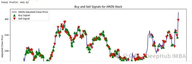
Amazon Stock Trading Signal Analysis

The experimental results show that the system performs well on stocks like Amazon, which have relatively stable volatility, accurately capturing price trends and making reasonable trading decisions.

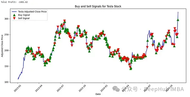
Tesla Stock Trading Signal Analysis

For stocks like Tesla, which have high volatility, the system shows certain limitations, indicating that optimizing trading strategies for high-volatility stocks remains a challenging research direction.

It is worth noting that the system demonstrated outstanding performance in trading NVIDIA stocks. This may be attributed to NVIDIA’s relatively stable upward trend in recent years due to increased GPU demand, allowing the system to better grasp trading opportunities.

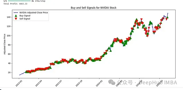
NVIDIA Stock Trading Signal Analysis

Conclusion

Through empirical research on three stocks with different volatility characteristics, we can see:

The system exhibits differentiated adaptability to different market environments. On relatively stable stocks like Amazon, the model can capture price trends well; while on high-volatility stocks like Tesla, the system’s performance is somewhat limited.

The combination of SSDA and LSTM-AE can effectively extract both static and dynamic features of the market, as fully validated by the trading results of NVIDIA stocks. Especially in the presence of clear market trends, the system demonstrates strong decision accuracy.

Through a multidimensional reward calculation mechanism, the system maintains effective risk control while pursuing returns, as reflected in the timing of trading signals and position management.

Limitations Analysis

Despite achieving certain results, there are still areas for improvement:

1. Adaptability to high-volatility market environments needs enhancement;
2. The model’s stability during periods of market turbulence needs further strengthening;

3. There may be information loss issues during feature extraction.

Future Research Directions

Based on the findings and limitations of this study, future research can unfold in the following directions:

1. Feature Engineering Optimization

• Introduce more market microstructure features
• Explore new feature fusion methods
• Research the application of attention mechanisms in feature extraction

• Design more complex neural network structures to enhance feature extraction capabilities
• Explore modeling methods that mix multiple time scales
• Research the application of ensemble learning in quantitative trading

• Develop more refined risk assessment metrics
• Research dynamic risk adjustment mechanisms

• Explore risk management methods at the portfolio level

Practical Value

The methodology and empirical results of this paper provide new insights for the design and implementation of quantitative trading systems. Especially in the context of an increasingly complex market environment, the application value of hybrid deep learning architectures deserves further exploration. With continuous optimization and improvement, such systems are expected to play a greater role in real trading environments.

As deep learning technologies continue to evolve and computational capabilities improve, similar hybrid architecture systems will have broad application prospects in the field of quantitative trading.