
Source: DeepHub IMBA


This article is about 1300 words long, and it is recommended to read it in 5 minutes.
This paper treats heart sound signals as speech signal processing and achieves good results.
This is a very interesting paper that proposes two heart rate sound classification models based on the log-mel spectrogram of heart sound signals. As we know, spectrograms are widely used in speech recognition. This paper treats heart sound signals as speech signal processing and achieves good results.
The heart sound signals are framed to a consistent length, extracting their log-mel spectrogram features. The paper proposes two deep learning models: Long Short-Term Memory (LSTM) and Convolutional Neural Network (CNN), to classify heart sounds based on the extracted features.
Heart Sound Dataset
Imaging diagnostics include cardiac magnetic resonance imaging (MRI), CT scans, and myocardial perfusion imaging. The drawbacks of these technologies are also evident, requiring high standards for modern machinery and professionals, and having long diagnostic times.
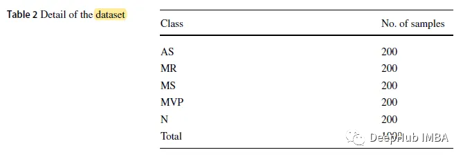
The paper uses a public dataset consisting of 1000 .wav format signal samples, with a sampling frequency of 8 kHz. The dataset is divided into 5 categories, including 1 normal category (N) and 4 abnormal categories: Aortic Stenosis (AS), Mitral Regurgitation (MR), Mitral Stenosis (MS), and Mitral Valve Prolapse (MVP).
Aortic Stenosis (AS) refers to the aortic valve being too small, narrowed, or stiff. The typical noise of aortic stenosis is a high-pitched “diamond” sound.
Mitral Regurgitation (MR) means that the heart’s mitral valve does not close properly, causing blood to flow back into the heart instead of being pumped out. When auscultating the fetal heart, S1 may be very low (sometimes very loud). Until S2, the volume of the noise increases. A short, rumbling diastolic murmur can be heard due to the rapid flow of the mitral valve after S3.
Mitral Stenosis (MS) refers to the mitral valve being damaged and unable to open fully. Heart sound auscultation shows an early S1 accentuation in mitral stenosis, and S1 softens in severe mitral stenosis. As pulmonary hypertension develops, S2 sound will be accentuated. Patients with pure multiple sclerosis have almost no left ventricular S3.
Mitral Valve Prolapse (MVP) refers to the mitral valve leaflets prolapsing into the left atrium during the heart’s contraction phase. MVP is usually benign, but complications include mitral regurgitation, endocarditis, and chord rupture. Signs include a mid-systolic click and late systolic murmur (if regurgitation is present).
Preprocessing and Feature Extraction
Sound signals have different lengths. Therefore, it is necessary to fix the sampling rate of each recording file. The length is trimmed to ensure that the sound signal contains at least one complete cardiac cycle. An adult’s heart beats 65-75 times per minute, with a heartbeat cycle of about 0.8 seconds, so the signal samples are trimmed to segments of 2.0 seconds, 1.5 seconds, and 1.0 seconds.
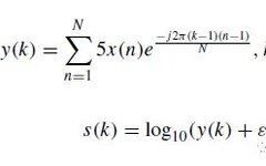
Based on the Discrete Fourier Transform (DFT), the raw waveform of the heart sound signal is converted into a log-mel spectrogram. The DFT y(k) of the sound signal is defined as Eq.(1), and the log-mel spectrogram s is defined as Eq.(2).

In the formula, N is the length of vector x, and ε = 10^(- 6) is a small offset. The waveform and log-mel spectrogram of some heart sound samples are shown below:

Deep Learning Models
1. LSTM

The LSTM model is designed with 2 layers directly connected, followed by 3 fully connected layers. The third fully connected layer feeds into a softmax classifier.
2. CNN Model
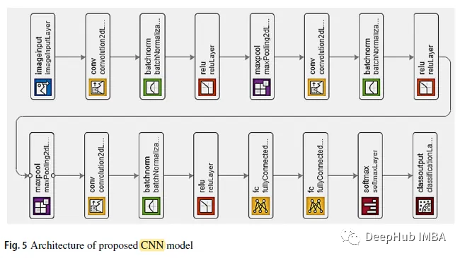
As shown in the figure, after the first two convolutional layers is an overlapping max pooling layer. The third convolutional layer is directly connected to the first fully connected layer. The second fully connected layer provides input to the softmax classifier with five class labels. BN and ReLU are used after each convolutional layer.
3. Training Details
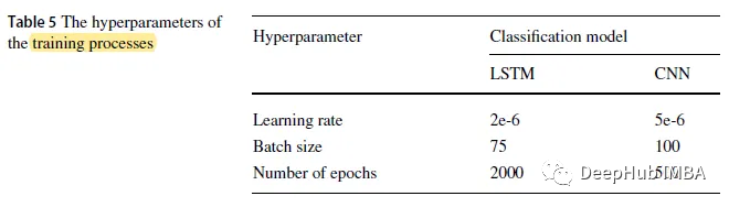
Results

The training set contains 70% of the entire dataset, and the test set contains the remaining part.
When the duration of the CNN model segment is 2.0 seconds, the highest accuracy is 0.9967; the lowest accuracy of the LSTM model with a segment time of 1.0 seconds is 0.9300.
The overall accuracy of the CNN model is 0.9967, 0.9933, and 0.9900 for segment durations of 2.0 seconds, 1.5 seconds, and 1.0 seconds, respectively, while the corresponding numbers for the LSTM model are 0.9500, 0.9700, and 0.9300.
The CNN model has higher prediction accuracy than the LSTM model across all time segments.
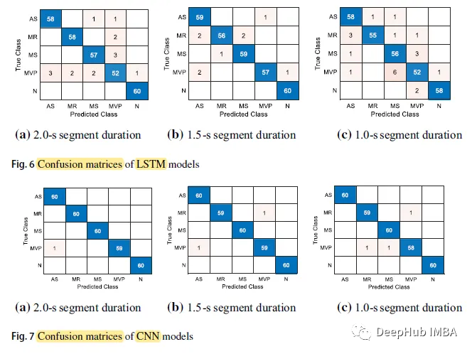
The confusion matrix is as follows:

The prediction accuracy for the N class (Normal) is the highest, reaching 60 out of 5 cases, while the MVP class has the lowest prediction accuracy across all cases.
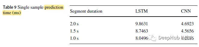
The input time length for the LSTM model is 2.0 seconds, with the longest prediction time being 9.8631 ms. The CNN model with a classification time of 1.0 seconds has the shortest prediction time of 4.2686 ms.
Compared to other SOTA models, some studies have very high accuracy, but these studies only conducted two categories (normal and abnormal), while this study is divided into five categories.
Compared to other studies using the same dataset (0.9700), this paper has significantly improved, achieving a maximum accuracy of 0.9967.