Hello everyone, I am Hua Ge. This article systematically and comprehensively organizes the introduction and algorithm principles of various deep learning models.
At the beginning of the article, let me first introduce our company’s popular business. If you have any needs or ideas, feel free to chat!

1 Main Text
Deep learning methods utilize neural network models for advanced pattern recognition and automatic feature extraction, achieving significant results in the field of data mining in recent years. Common models include not only the basic DNN but also RNN, LSTM, GRU, CNN, Attention, and Mix hybrid models.
Compared to complex feature engineering in machine learning, deep learning models only require data preprocessing, network structure design, and hyperparameter tuning to output prediction results. Deep learning algorithms can automatically learn patterns and trends in sequential data, demonstrating excellent expressive power for complex nonlinear patterns. When applying these models, one must consider data stationarity and periodicity, choose appropriate models and parameters, conduct training and testing, and perform tuning and validation.
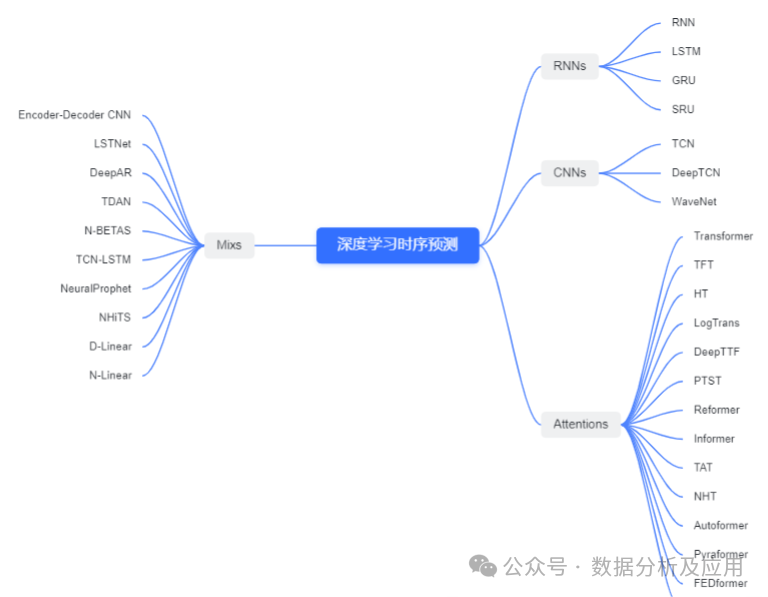
2 Overview of Deep Learning Algorithms
2.1 RNN Class
In RNNs, the input at each moment and the states from previous moments are carefully mapped and merged into a hidden state, allowing for precise prediction of the output at the next moment based on the current input and previous states. A notable feature of RNNs is their powerful capability to handle variable-length sequence data, making them particularly adept at processing time series data and providing unique advantages for time series forecasting. Additionally, to further enhance the model’s expressive and memory capabilities, RNNs can cleverly integrate advanced gating mechanisms such as LSTM, GRU, and SRU to construct more robust and flexible neural network models.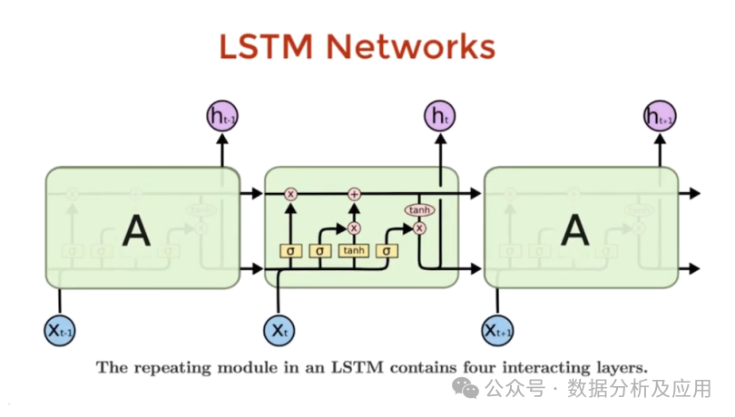
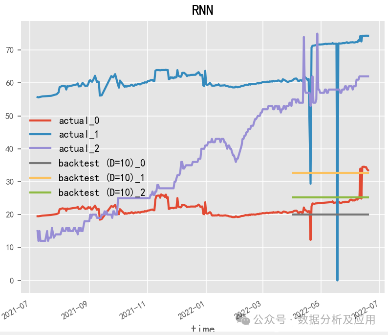
2.1.1 RNN (1990)
Paper: Finding Structure in Time
The RNN (Recurrent Neural Network) is a powerful deep learning model widely used in time series forecasting tasks. It effectively transmits historical information to the future by unfolding the neural network over the time dimension, thus addressing the inherent temporal dependencies and dynamic changes in time series data. When constructing RNN models, LSTM and GRU models are particularly favored as they can tackle long sequence challenges and, through memory cells and gating mechanisms, precisely capture temporal dependencies in time series data.
2.1.2 LSTM (1997)
Paper: Long Short-Term Memory
LSTM (Long Short-Term Memory) is a commonly used recurrent neural network model, often employed in time series forecasting. Compared to the basic RNN model, LSTM has stronger memory and long-term dependency capabilities, allowing it to better handle temporal dependencies and dynamic changes in time series data. The design and parameter tuning of LSTM units are crucial as they can affect the model’s memory capability and long-term dependency ability, while parameter adjustments can influence prediction accuracy and robustness.
# LSTMmodel = RNNModel(model="LSTM",hidden_dim=60,dropout=0,batch_size=100,n_epochs=200,optimizer_kwargs={"lr": 1e-3}, # model_name="Air_RNN",log_tensorboard=True,random_state=42,training_length=20,input_chunk_length=60, # force_reset=True, # save_checkpoints=True,)2.1.3 GRU (2014)
Paper: Learning Phrase Representations using RNN Encoder–Decoder for Statistical Machine Translation
GRU (Gated Recurrent Unit) is a commonly used recurrent neural network model, whose structural characteristics are quite similar to that of LSTM, specifically designed to capture deep information in time series data. Compared to LSTM, GRU maintains the ability to handle temporal dependencies and dynamic changes while having a more streamlined number of parameters and faster computation speed. Its core lies in the exquisite design of the GRU unit and the fine-tuning of its parameters. The design of the GRU unit not only affects the model’s memory capability but also has a profound impact on its ability to capture long-term dependencies; precise adjustments of parameters directly relate to the model’s prediction accuracy and robustness.
GRUmodel = RNNModel(model="GRU",hidden_dim=60,dropout=0,batch_size=100,n_epochs=200,optimizer_kwargs={"lr": 1e-3}, # model_name="Air_RNN",log_tensorboard=True,random_state=42,training_length=20,input_chunk_length=60, # force_reset=True, # save_checkpoints=True,)2.1.4 SRU (2018)
Paper: Simple Recurrent Units for Highly Parallelizable Recurrence
SRU (Simple Recurrent Unit) is an innovative recurrent neural network model designed for efficient matrix computation, specifically developed for processing time series data. Compared to traditional LSTM and GRU models, SRU significantly reduces the number of parameters while maintaining efficient temporal dependence handling and dynamic change capture, thereby enhancing computation speed. The performance of the SRU model depends on the cleverness of its unit design and the precise adjustments of parameters. A well-designed SRU unit can strengthen the model’s memory capability and long-term dependency capture ability, while fine-tuning parameters plays a critical role in the model’s prediction accuracy and robustness.
2.2 CNN Class
CNNs, with their unique convolutional and pooling layer structures, can automatically extract key features from time series data, achieving efficient and accurate temporal predictions. In practical applications, we need to convert one-dimensional time series data into two-dimensional matrix form and use CNN’s convolution and pooling operations for feature extraction and compression. Finally, predictions are made through fully connected layers. Compared to traditional time series forecasting methods, CNNs have gradually become leaders in the field due to their powerful feature learning capabilities, efficient computational efficiency, and excellent prediction accuracy.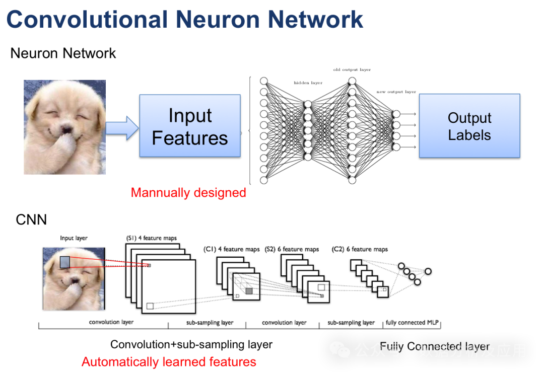
2.2.1 WaveNet (2016)
Paper: WAVENET: A GENERATIVE MODEL FOR RAW AUDIO
WaveNet, a breakthrough neural network model proposed by the DeepMind team in 2016, centers on simulating the waveform characteristics of audio signals using convolutional neural networks. By integrating residual connections and gated convolution operations, WaveNet significantly enhances the model’s representational capabilities. In addition to excelling in speech generation, WaveNet is also suitable for time series forecasting tasks. In practical applications, we can treat time series as one-dimensional vectors and input them into the WaveNet model to achieve precise predictions for future time steps.
When constructing the WaveNet model, the design of convolutional layers and parameter adjustments are critical. Well-designed convolutional layers can enhance the model’s expressive capability and generalization ability, while precise parameter tuning directly relates to the model’s prediction accuracy and stability.
2.2.2 TCN (2018)
TCN, as a temporal convolutional network, achieves efficient processing of time series data by introducing causal convolutions and residual connections among other innovative structures. It not only captures long-term dependencies in sequences but also possesses excellent parallel computing capabilities, greatly improving the efficiency and accuracy of time series forecasting. In practical applications, TCN exhibits strong potential and broad application prospects, bringing new breakthroughs and development directions to the field of time series forecasting. Paper: An Empirical Evaluation of Generic Convolutional and Recurrent Networks for Sequence Modeling
TCN (Temporal Convolutional Network) is an innovative time series forecasting algorithm built on convolutional neural networks, aimed at solving the problems of gradient vanishing and excessive computational complexity often encountered by traditional RNNs when processing long sequences. Compared to traditional RNNs and other sequence models, TCN can more efficiently capture long-term dependencies while exhibiting excellent parallel computing capabilities.
The TCN model consists of carefully designed convolutional layers and residual connections. Each convolutional layer is responsible for extracting deep features from the sequence data and passing them to the next layer, achieving a step-by-step abstraction and feature extraction of the data. The model also cleverly incorporates residual connection techniques similar to ResNet, effectively reducing gradient vanishing and model degradation issues. Moreover, the application of dilated convolutions further expands the receptive field of the convolutional kernels, enhancing the model’s robustness and accuracy.
The prediction process of this model is orderly, with specific steps as follows:
-
Input Layer: Responsible for receiving the input of time series data, laying the foundation for subsequent processing.
-
Convolution Layer: Utilizing one-dimensional convolution techniques to extract and abstract features from the input data. Each convolution layer contains multiple convolution kernels, capable of capturing time series patterns at different scales.
-
Residual Connection: Borrowing from ResNet’s design philosophy, the residual connection technique effectively combines the output of the convolution layer with its input, alleviating gradient vanishing and model degradation issues, thus enhancing model stability.
-
Repeated Stacking: By repeatedly stacking multiple convolution layers and residual connections, the model can progressively extract abstract features from the time series data.
-
Pooling Layer: A global average pooling layer is set deep within the model to average all feature vectors, obtaining a fixed-length feature vector.
-
Output Layer: After processing through fully connected layers, the output of the pooling layer is transformed into the predicted values of the time series.
The advantages of the TCN model are significant:
-
It can effectively handle long sequence data, demonstrating excellent parallel performance.
-
By utilizing advanced technologies such as residual connections and dilated convolutions, it effectively avoids gradient vanishing and overfitting phenomena.
-
Compared to traditional RNN models, the TCN model exhibits outstanding performance in both computational efficiency and prediction accuracy.
2.2.3 DeepTCN (2019)
Paper: Probabilistic Forecasting with Temporal Convolutional Neural Network
Code: deepTCN
DeepTCN (Deep Temporal Convolutional Networks) is a deep learning-based time series forecasting model that deepens and expands the traditional TCN model. This model utilizes a set of carefully designed 1D convolutional layers and max pooling layers to deeply process time series data, achieving feature extraction through layer stacking. In DeepTCN, each convolution layer is equipped with multiple 1D convolution kernels and activation functions, while also integrating residual connections and batch normalization techniques to accelerate the training process of the model.
The training process of the DeepTCN model is rigorous and efficient, consisting of the following steps:
-
Data Preprocessing: Standardizing and normalizing the raw time series data to eliminate the impact of different feature scales on model training.
-
Model Construction: Utilizing deep learning frameworks (such as TensorFlow, PyTorch, etc.) to construct a DeepTCN model containing multiple 1D convolutional layers and max pooling layers.
-
Model Training: Using the training dataset to finely train the DeepTCN model, accurately measuring the model’s prediction performance through loss functions (such as MSE, RMSE, etc.). During the training process, optimization algorithms (such as SGD, Adam, etc.) are employed to adjust model parameters, and techniques like batch normalization and DeepTCN are used to enhance the model’s generalization ability.
-
Model Evaluation: Using the testing dataset to comprehensively evaluate the trained DeepTCN model, calculating and comparing various performance indicators such as Mean Absolute Error (MAE), Mean Absolute Percentage Error (MAPE), etc.
2.3 Attention Class
The attention mechanism serves as a core method for extracting important features from sequence input data, playing a crucial role in the field of time series forecasting. The attention mechanism can precisely focus on key parts of time series data, providing the model with more valuable information, thereby significantly improving prediction accuracy. When using attention for time series forecasting, we must leverage its ability to adaptively adjust the weights of different parts of the input data, allowing the model to concentrate more on core information while diminishing the interference of irrelevant information. The attention mechanism is not only applicable to sequence models like RNNs but also performs excellently in non-sequence models like CNNs, making it a research focus in the current time series forecasting field.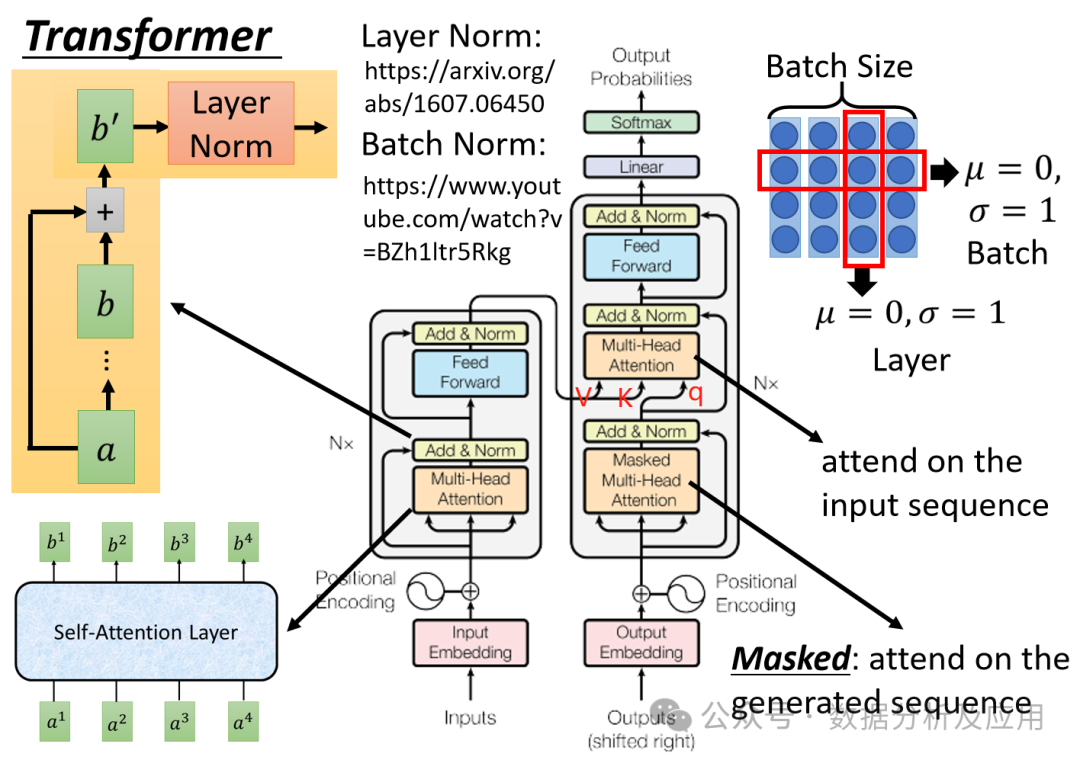
2.3.1 Transformer (2017)
Paper: Attention Is All You Need
The Transformer is a neural network model that has excelled in the field of natural language processing (NLP), fundamentally serving as a sequence-to-sequence (seq2seq) mapping model. The Transformer treats each position in the sequence as an independent vector and utilizes multi-head self-attention mechanisms along with feedforward neural networks to deeply explore the long-range dependencies contained in the sequence, ensuring that the model can flexibly handle sequences of varying lengths.
In time series forecasting tasks, the Transformer model cleverly transforms the time steps of the input sequence into positional information, expressing the features of each time step in vector form. With the encoder-decoder framework, the Transformer model can efficiently complete prediction tasks. Specifically, we input the first N time steps of the prediction target as the encoder’s input while using the subsequent M time steps of the prediction target as the decoder’s input, utilizing the encoder-decoder framework for precise predictions. Both the encoder and decoder are composed of multiple stacked Transformer modules, each consisting of multi-head self-attention layers and feedforward neural network layers.
During the training phase, we can select classic loss functions such as Mean Squared Error (MSE) or Mean Absolute Error (MAE) to measure the model’s prediction performance, while also continuously adjusting model parameters using optimization algorithms such as Stochastic Gradient Descent (SGD) or Adam to optimize performance. Additionally, to improve training efficiency and model performance, we can adopt advanced techniques such as learning rate adjustments and gradient clipping.
model = TransformerModel(input_chunk_length=30,output_chunk_length=15,batch_size=32,n_epochs=200, # model_name="air_transformer",nr_epochs_val_period=10,d_model=16,nhead=8,num_encoder_layers=2,num_decoder_layers=2,dim_feedforward=128,dropout=0.1,optimizer_kwargs={"lr": 1e-2},activation="relu",random_state=42, # save_checkpoints=True, # force_reset=True,)2.3.2 TFT (2019)
Paper: Temporal Fusion Transformers for Interpretable Multi-horizon Time Series Forecasting
TFT (Temporal Fusion Transformers) is a Transformer model that integrates temporal fusion, providing a powerful tool for interpretable multi-scale time series forecasting. By introducing a temporal fusion mechanism, TFT effectively enhances the model’s prediction accuracy in complex time series data. This model can address the forecasting needs of single time scales while also handling multi-scale time series forecasting problems, further expanding its application scope. Moreover, the strong interpretability of the TFT model makes the prediction results more convincing, providing strong support for decision-making. TFT (Transformer-based Time Series Forecasting) is a time series forecasting method based on the Transformer model, ingeniously proposed by Google’s DeepMind team in 2019. Its core idea is to cleverly integrate temporal feature embeddings and modality embeddings, allowing the Transformer model to more accurately capture periodic and trend features in time series data while comprehensively considering external influencing factors (such as temperature, holidays, etc.) for forecasting.
The TFT method consists of two main phases: training and forecasting. During the training phase, this method uses rich training data to refine the Transformer model, employing strategies such as random masking and adaptive learning rate adjustments to effectively enhance the model’s robustness and training efficiency. In the forecasting phase, the trained model can accurately predict future time series data trends.
Compared to traditional time series forecasting methods, the TFT method has distinct advantages:
-
It can flexibly respond to time series data of different scales, as the Transformer model excels at capturing both global and local features of time series.
-
It can comprehensively consider time series data and external influencing factors, thereby improving prediction accuracy.
-
It eliminates the need for manual feature extraction, as it can learn the prediction model directly through end-to-end training.
HT (Hierarchical Transformer)
As another leader in the field of time series forecasting, the HT model was proposed by a research team from the Chinese University of Hong Kong in 2019. This model adopts a hierarchical structure aimed at processing time series data with multiple time scales. Through an adaptive attention mechanism, the HT model can accurately capture features across different time scales, significantly enhancing prediction performance and generalization ability.
The HT model consists of two core components: a multi-scale attention module and a prediction module. In the multi-scale attention module, the HT model employs an adaptive multi-head attention mechanism to effectively fuse features across different time scales, forming a unified feature representation. In the prediction module, the model finely predicts the feature representation through fully connected layers and outputs the final prediction results.
The excellence of the HT model lies in its ability to adaptively process multi-time scale time series data and accurately capture features through the adaptive multi-head attention mechanism. This allows it to demonstrate outstanding prediction performance and good generalization ability in time series forecasting tasks, while also possessing good interpretability, making it suitable for various time series forecasting scenarios.
As for LogTrans (2019), it is an advanced method aimed at enhancing locality and breaking the memory bottleneck of the Transformer in time series forecasting. This method is discussed in depth in the paper “Enhancing the Locality and Breaking the Memory Bottleneck of Transformer on Time Series Forecasting” and provides the implementation code for Autoformer, offering new ideas and directions for research and applications in the field of time series forecasting. LogTrans proposes an improved Transformer method for time series forecasting that cleverly combines convolutional self-attention mechanisms and LogSparse Transformer technology. The convolutional self-attention mechanism generates queries and keys with causal convolution characteristics, successfully integrating local environments into the attention mechanism, enhancing the model’s ability to capture local features in time series data. Meanwhile, LogSparse Transformer serves as an efficient variant of the Transformer, optimizing memory usage and significantly reducing the memory costs of modeling long time series, making the model more efficient when processing large-scale time series data. The introduction of LogTrans effectively addresses the two major issues of the Transformer in time series forecasting caused by position-agnostic attention and memory bottlenecks.
2.3.5 DeepTTF (2020)
DeepTTF (Deep Temporal Transformational Factorization) is an advanced time series forecasting algorithm proposed by researchers at UCLA, based on deep learning and matrix factorization techniques. This method cleverly decomposes time series into multiple independent time segments and deeply analyzes the potential relationships within each time segment using matrix factorization techniques, significantly improving the model’s prediction accuracy and interpretability.
The core architecture of the DeepTTF model consists of three key links: time segmentation, matrix factorization, and predictor. In the time segmentation phase, the model divides complex time series into multiple manageable subsequences for subsequent detailed processing. In the matrix factorization phase, DeepTTF employs advanced matrix factorization techniques to effectively reveal the complex interactions between time and features in the time series. Finally, the predictor utilizes multilayer perceptrons to make precise predictions for the decomposed subsequences, generating the final prediction results through clever combination strategies.
The uniqueness of the DeepTTF model lies in its strong ability to capture local patterns and analyze global trends, allowing it to maintain high prediction accuracy even when faced with complex and variable time series data. Additionally, this model supports a time-segment-based cross-validation strategy, further enhancing the model’s robustness and generalization ability, enabling it to perform excellently in various time series forecasting tasks.
2.3.6 PTST (2020)
PTST (Probabilistic Time Series Transformer) is an innovative time series forecasting algorithm proposed by Google Brain in 2020, based on the Transformer model and combined with probabilistic graphical models to improve the accuracy and reliability of time series forecasting. PTST effectively captures uncertainty and noise in time series data by introducing probabilistic graphical models, allowing the model to perform better when handling highly uncertain time series data.
The core architecture of the PTST model consists of two major modules: the sequence model and the probability model. The sequence model employs an advanced Transformer structure, achieving deep encoding and decoding of time series data through multi-layer self-attention mechanisms. The probability model innovatively incorporates Variational Autoencoders (VAE) and Kalman Filters (KF), working together on noise processing and smoothing optimization of time series data.
During the training process, PTST adopts a Maximum A Posteriori (MAP) estimation method, aiming to maximize the probability of the predicted results. In the forecasting phase, PTST utilizes Monte Carlo sampling methods to extract samples from the posterior distribution, generating a set of probability distributions to provide rich information support for decision-makers. Furthermore, PTST introduces loss functions such as Mean Squared Error and Negative Log Likelihood (NLL) to comprehensively assess the model’s prediction performance.
2.3.7 Reformer (2020)
Reformer is an efficient Transformer model proposed in 2020 that significantly reduces the consumption of computational and storage resources while maintaining the superior performance of the Transformer. Reformer achieves efficient processing of long sequences by introducing innovative techniques such as Locality-Sensitive Hashing (LSH) attention mechanisms and reversible layers.
The LSH attention mechanism is one of the core technologies of Reformer, which reduces the spatial complexity of attention calculations from O(n²) to O(n log n), significantly enhancing the model’s computational efficiency when processing long sequences. Additionally, the reversible layer technology allows the model to reduce memory usage during training, further alleviating the pressure on resource consumption.
The introduction of Reformer not only provides an efficient and high-performance solution for tasks such as time series forecasting but also injects new vitality into the development of the deep learning field. In the future, as data scales continue to expand and computational resources are continuously optimized, Reformer is expected to play an important role in more scenarios. Reformer, as a neural network structure based on the Transformer model, demonstrates broad application prospects in time series forecasting tasks. It can achieve precise predictions for future time steps through sampling, autoregression, multi-step forecasting, and integration with reinforcement learning. In this process, the model cleverly utilizes known historical time step information to ensure continuity and accuracy in predictions. Notably, Reformer enhances processing efficiency through the introduction of separable convolutions and reversible layers, achieving significant breakthroughs in prediction accuracy and demonstrating its efficient, accurate, and scalable performance. The birth of the Reformer model undoubtedly brings a new dimension and solution strategy for time series forecasting tasks.
2.3.8 Informer (2020)
Paper: Informer: Beyond Efficient Transformer for Long Sequence Time-Series Forecasting
Code: https://github.com/zhouhaoyi/Informer2020
Informer, a time series forecasting method based on the Transformer model, originates from the outstanding contributions of the Deep Learning and Computing Intelligence Laboratory at Peking University in 2020. It is not merely a simple improvement of the traditional Transformer model but incorporates numerous innovative structures and mechanisms to meet the complex demands of time series forecasting. The core idea of Informer is:
-
Utilizing Long Short-Term Memory (LSTM) encoder-decoder structures to effectively alleviate the challenges posed by long-term dependencies in time series.
-
Introducing an Adaptive Length Attention (AL) mechanism, enabling the model to flexibly capture key information across different time scales, enhancing prediction accuracy.
-
Integrating Multi-Scale Convolutional Kernels (MSCK) mechanisms to fully explore and utilize features across different time scales, thereby enhancing the model’s generalization ability.
-
Leveraging Generative Adversarial Networks (GAN) frameworks to further refine model performance and optimize prediction results through adversarial learning.
During the training phase, Informer supports various loss functions to guide model learning and employs the Adam optimization algorithm to precisely adjust model parameters. In the forecasting phase, Informer utilizes sliding window techniques to achieve precise predictions for future time points. Through validation and comparison across multiple time series forecasting datasets, Informer demonstrates outstanding performance in prediction accuracy, training speed, and computational efficiency.
2.3.9 TAT (2021)
TAT (Temporal Attention Transformer) is a time series forecasting algorithm proposed by the Intelligent Science Laboratory at Peking University, which innovatively expands upon the traditional Transformer model. Its core lies in introducing a temporal attention mechanism to more accurately capture dynamic changes in time series.
The TAT model inherits the classic design of the Transformer structure, including multiple Encoder and Decoder layers. Each Encoder layer integrates multi-head self-attention mechanisms and feedforward networks to effectively extract key information from the input sequence. The Decoder layer, on the other hand, increases attention to the Encoder’s output based on the self-attention mechanism and generates the final prediction results through feedforward networks. Notably, the TAT model innovatively incorporates a temporal attention mechanism into the multi-head attention mechanism. This mechanism allows the model to include time step information as an additional feature, enabling it to more sensitively capture dynamic changes in time series. This design not only enhances the model’s ability to model complex time series but also lays a solid foundation for its excellent performance in time series forecasting tasks.
Additionally, the TAT model employs incremental training techniques to improve the model’s training efficiency and prediction performance. This technique allows the model to achieve faster and more accurate convergence within limited time and computational resources, thus meeting the practical demand for time series forecasting.
2.3.10 NHT (2021)
NHT, as a cutting-edge time series forecasting method, has received widespread attention in recent years. Its uniqueness lies in combining the advantages of deep learning and traditional time series analysis methods, providing a new solution for time series forecasting tasks. The NHT model can effectively capture complex dynamic changes in time series and possesses strong feature extraction and pattern recognition capabilities. Through continuous learning and optimization, the NHT model can demonstrate excellent performance in various time series forecasting scenarios. With further research and the ongoing development of technology, the NHT model is expected to play an increasingly important role in the future of time series forecasting. Paper: Nested Hierarchical Transformer: Towards Accurate, Data-Efficient, and Interpretable Visual Understanding
NHT (Nested Hierarchical Transformer) is a deep learning algorithm specifically applied to time series forecasting. This algorithm cleverly integrates a nested hierarchical transformer structure with multi-level nested self-attention mechanisms and a temporal importance assessment mechanism to achieve precise insights and predictions for time series data. The NHT model enhances the traditional self-attention mechanism through upgrades and optimizations, introducing more hierarchical structures while employing a dynamic regulatory mechanism, namely the temporal importance assessment mechanism, to effectively control the weight distribution of different levels during the prediction process, significantly enhancing prediction performance. This algorithm has achieved remarkable results in various time series forecasting tasks, fully demonstrating its outstanding potential and infinite possibilities in the field of time series forecasting.
2.3.11 Autoformer (2021)
Paper: Autoformer: Decomposition Transformer Based on Autocorrelation for Long-Term Sequence Forecasting
Code: https://github.com/thuml/Autoformer
AutoFormer is an innovative time series forecasting model based on the Transformer structure. Compared to traditional models like RNNs and LSTMs, it has the following significant advantages:
-
Self-Attention Mechanism: AutoFormer cleverly employs self-attention mechanisms to simultaneously capture the complex global and local relationships in time series, effectively avoiding the gradient vanishing issues that may arise during long sequence training.
-
Transformer Structure: AutoFormer fully utilizes the parallel computing ability of the Transformer structure, greatly enhancing training efficiency to meet the demands of modern large-scale data processing.
-
Multi-Task Learning Capability: AutoFormer supports multi-task learning paradigms, allowing for simultaneous predictions of multiple time series, thereby improving prediction accuracy while achieving efficient processing.
The structural design of the AutoFormer model is exquisite, consisting of two core components: the encoder and the decoder. The encoder deeply extracts features from the input sequence by stacking multiple self-attention layers and feedforward neural network layers; the decoder similarly transforms the encoder’s output into precise prediction sequences. Additionally, AutoFormer introduces cross-time-step attention mechanisms, enabling the encoder and decoder to adaptively adjust time step lengths as needed. Overall, AutoFormer is a highly efficient and precise time series forecasting model suitable for various complex and variable time series forecasting tasks.
2.3.12 Pyraformer (2022)
Paper: Pyraformer: Low Complexity Pyramid Attention Mechanism for Long-Range Time Series Modeling and Forecasting
Code: https://github.com/ant-research/Pyraformer
Pyraformer is a novel time series forecasting model that centers on a unique low-complexity pyramid attention mechanism, providing an efficient and accurate solution for long-range time series modeling and forecasting. This model constructs a pyramid-style attention structure to achieve fine capture and processing of information across different time scales, effectively addressing the challenges of long sequence forecasting. The excellent performance of Pyraformer allows it to stand out in various time series forecasting tasks, becoming a research hotspot and frontier direction in this field. The Ant Research Institute recently proposed Pyraformer, which is a Transformer model based on pyramid attention, aimed at bridging the gap between capturing long-distance dependencies and achieving low spatiotemporal complexity. Specifically, Pyraformer develops a pyramid graph and conveys attention-based information, as illustrated in the figure (d). In this figure, edges are cleverly divided into two groups: inter-scale connections and intra-scale connections. Inter-scale connections construct multi-resolution representations of the original sequence, where nodes at the finest scale correspond precisely to time points in the original time series (e.g., hourly observations), while nodes at coarser scales represent lower-resolution features (e.g., daily, weekly, and monthly patterns). These potential coarse-scale nodes are initially introduced through innovative coarse-scale construction modules. On the other hand, intra-scale edges cleverly capture temporal correlations at each resolution by closely connecting adjacent nodes. Thus, Pyraformer efficiently captures these behaviors at coarser resolutions, shortening the length of signal traversal paths, and providing a concise and effective representation for long-range time dependencies between distant locations. Additionally, through sparse adjacent intra-scale connections, this model models different ranges of temporal dependencies at different scales, significantly reducing computational costs.
2.3.13 FEDformer (2022)
Paper: FEDformer: Frequency Enhanced Decomposed Transformer for Long-term Series Forecasting
Code: https://github.com/MAZiqing/FEDformer
FEDformer is an innovative Transformer neural network structure specifically designed for distributed time series forecasting tasks. This model cleverly decomposes time series data into multiple small chunks and significantly accelerates the training process through distributed computing. FEDformer not only introduces local attention mechanisms and reversible attention mechanisms, allowing the model to more precisely capture local features in time series data, but also possesses outstanding computational efficiency. Furthermore, it supports advanced features such as dynamic partitioning, asynchronous training, and adaptive chunking, endowing the model with greater flexibility and scalability.
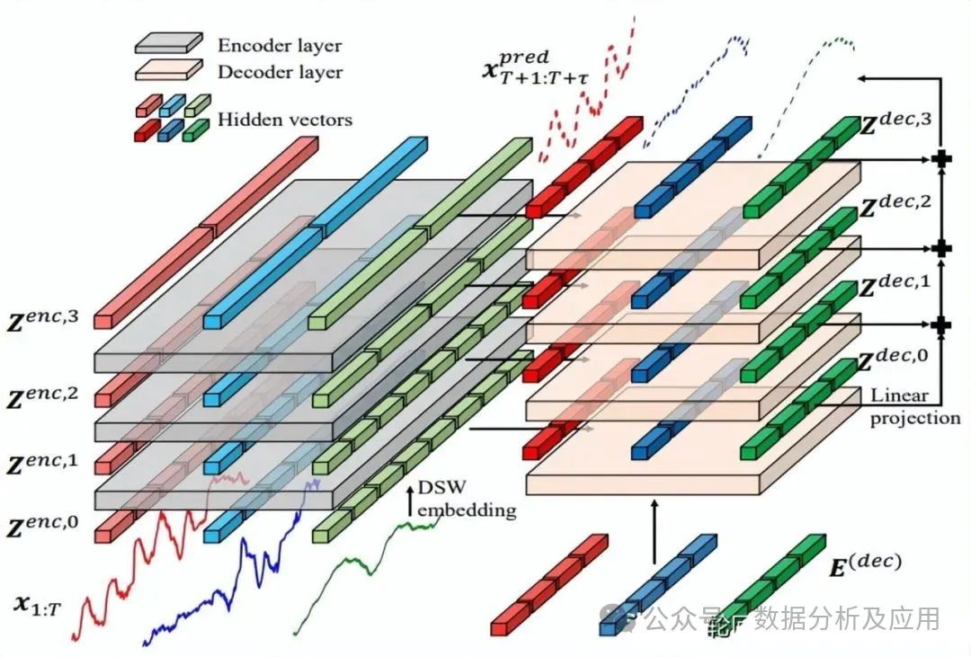
2.3.14 Crossformer (2023)
Paper: Crossformer: Transformer Utilizing Cross-Dimension Dependency for Multivariate Time Series Forecasting
Code: https://github.com/Thinklab-SJTU/Crossformer
Crossformer innovatively proposes a new hierarchical Encoder-Decoder architecture, composed of the left Encoder (gray) and the right Decoder (light orange), integrating innovative elements such as Dimension-Segment-Wise (DSW) embedding, Two-Stage Attention (TSA) layers, and Linear Projection. This design allows Crossformer to fully leverage cross-dimensional dependencies, bringing revolutionary performance improvements to multivariate time series forecasting tasks.
2.4 Mix Class
By integrating algorithms such as ETS, autoregression, RNN, CNN, and Attention, we can fully leverage their respective advantages, thereby significantly enhancing the accuracy and stability of time series forecasting. This clever fusion strategy is often referred to as a “hybrid model” in the industry.
In hybrid models, RNNs uniquely excel in automatically capturing the intricate long-term dependencies in time series data; CNNs, with their exceptional feature extraction capabilities, are adept at mining local and spatial features within time series data; while the Attention mechanism, with its flexible adaptability, precisely focuses on key parts of time series data. By organically combining these algorithms, we can construct more robust and accurate time series forecasting models.
In practical applications, we can flexibly choose suitable algorithm fusion methods based on different time series forecasting scenarios and meticulously tune and optimize the models to ensure they achieve optimal performance.
2.4.1 Encoder-Decoder CNN (2017)
Paper: Deep Learning for Precipitation Nowcasting: A Benchmark and A New Model
Encoder-Decoder CNN is an advanced model designed for time series forecasting tasks, cleverly combining encoders and decoders with convolutional neural networks. In this model, the encoder is responsible for deeply mining the inherent features of time series data, while the decoder generates future time series data based on these features.
The specific process for making time series predictions using the Encoder-Decoder CNN model is as follows:
-
First, historical time series data is inputted, and convolutional layers are used to extract features.
-
Next, the feature sequence outputted by the convolutional layer is passed to the encoder, which gradually reduces the dimensionality of the features through pooling operations while preserving the encoder’s state vector.
-
Then, the encoder’s state vector is inputted into the decoder, which gradually reconstructs and generates future time series data through deconvolution and upsampling operations.
-
Finally, necessary post-processing, such as mean removal or normalization, is performed on the decoder’s output to obtain the final accurate and reliable prediction results.
It is worth noting that during the training process of the Encoder-Decoder CNN model, appropriate loss functions (such as mean squared error or cross-entropy) should be selected, and hyperparameters adjusted according to actual needs. Additionally, cross-validation and other technical measures should be employed to evaluate and optimize the model, enhancing its generalization ability.
2.4.2 LSTNet (2018)
Paper: Modeling Long- and Short-Term Temporal Patterns with Deep Neural Networks
LSTNet is a deep learning model specifically designed for time series forecasting, with its full name being Long- and Short-term Time-series Networks. This model cleverly integrates Long Short-Term Memory networks (LSTM) and one-dimensional convolutional neural networks (1D-CNN), allowing it to simultaneously process long-term and short-term information in time series and effectively capture seasonal and cyclical changes within the sequences. LSTNet was first proposed in 2018 by Guokun Lai and others from the Institute of Computing Technology, Chinese Academy of Sciences.
The core idea of the LSTNet model is to utilize CNNs for feature extraction from time series data, subsequently feeding these features into LSTMs for in-depth sequence modeling. Additionally, LSTNet introduces an adaptive weight learning mechanism to flexibly adjust the weights of long-term and short-term time series information in predictions. The model’s input is a time series matrix shaped as (T, d), where T represents the number of time steps and d represents the feature dimension at each time step. The model’s output is a prediction vector of length H, where H denotes the number of time steps to be predicted. During training, LSTNet employs Mean Squared Error (MSE) as the loss function and optimizes through backpropagation.
2.4.3 TDAN (2018)
Paper: TDAN: Temporal Difference Attention Network for Precipitation Nowcasting
TDAN (Temporal Difference Attention Network) is an innovative model designed for precipitation nowcasting tasks, fully leveraging the advantages of temporal differences and attention mechanisms. TDAN captures temporal difference information in time series data and combines it with attention mechanisms to focus on key time periods and regions, achieving precise predictions of precipitation conditions. The outstanding performance of TDAN demonstrates its potential and application value in the field of time series forecasting. TDAN (Time-aware Deep Attentive Network) is an advanced deep learning algorithm specifically designed for time series forecasting. It cleverly captures temporal features in time series by integrating convolutional neural networks with attention mechanisms. Compared to traditional convolutional neural networks, TDAN can more efficiently utilize the temporal information in time series data, significantly enhancing the accuracy of time series predictions.
Specifically, the time series forecasting process of the TDAN algorithm can be summarized in the following steps:
-
First, historical time series data is inputted, and convolutional layers are used to deeply extract the core features of the time series.
-
Next, the feature sequence outputted by the convolutional layer is passed to the attention mechanism, which calculates a weighted feature vector based on the weight information tightly related to the current prediction from the historical data.
-
Finally, the weighted feature vector is sent to fully connected layers for precise and efficient predictions.
It is important to note that during the training process of the TDAN algorithm, appropriate loss functions (such as mean squared error) should be selected, and hyperparameters adjusted according to actual needs. Additionally, to enhance the model’s generalization ability, advanced techniques such as cross-validation should be employed for model evaluation and selection.
One major advantage of the TDAN algorithm is its ability to adaptively focus on the parts of historical data that are highly relevant to the current prediction, significantly improving the accuracy of time series forecasting. Furthermore, TDAN can effectively handle missing values and anomalies in time series data, demonstrating outstanding robustness.
2.4.4 DeepAR (2019)
Paper: DeepAR: Probabilistic Forecasting with Autoregressive Recurrent Networks
DeepAR is an innovative autoregressive recurrent neural network that cleverly combines recurrent neural networks (RNN) with autoregressive AR methods, focusing on predicting scalar (one-dimensional) time series. In many practical scenarios, we often face a series of similar time series with representative units. DeepAR can effectively integrate these multiple similar time series data, such as sales data for different flavors of instant noodles, capturing the interrelations within different time series through deep recurrent neural networks. This multi-target setting helps improve overall prediction accuracy.
DeepAR can generate multi-step prediction results for selectable time spans, with each time node prediction being probabilistic. By default, it outputs three values: P10, P50, and P90. Here, P10 indicates there is a 10% chance that the actual value will be less than the predicted value P10. By providing probabilistic predictions, we can either combine the three values to give a deterministic prediction or utilize the prediction intervals from P10 to P90 to formulate more flexible decision-making plans.
2.4.5 N-BEATS (2020)
Paper: N-BEATS: Neural Basis Expansion Analysis for Interpretable Time Series Forecasting
Code Repository: https://github.com/amitesh863/nbeats_forecast
N-BEATS (Neural basis expansion analysis for interpretable time series forecasting) is a novel time series forecasting model based on neural networks, meticulously developed by Oriol Vinyals and others from the Google Brain team. N-BEATS employs learning-based basis functions to accurately represent time series data, significantly enhancing the model’s interpretability while maintaining high prediction accuracy. Moreover, the N-BEATS model innovatively combines stacked regression modules and inverse convolution modules to effectively address challenges posed by multi-scale time series data and long-term dependencies.
Through the following code example, we can easily create and configure an N-BEATS model:
model = NBEATSModel( input_chunk_length=30, output_chunk_length=15, n_epochs=100, num_stacks=30, num_blocks=1, num_layers=4, dropout=0.0, activation='ReLU')By adjusting the model parameters according to specific task requirements, we can achieve optimal prediction results. 2.4.6 TCN-LSTM (2021)
Paper: Research on Detecting Anomalies in Time Series Data Using LSTM and TCN Models
TCN-LSTM, as an advanced model that integrates Temporal Convolutional Network (TCN) and Long Short-Term Memory (LSTM), demonstrates outstanding performance in time series forecasting tasks. In this collaborative model, TCN layers and LSTM layers each play their roles, jointly capturing long-term and short-term features of time series. Specifically, the TCN layer processes historical time series data, accurately extracting key features in the short term; then, these processed feature sequences are inputted into the LSTM layer, allowing it to leverage its strengths to delve into the long-term dependencies hidden within the time series; finally, the feature vectors outputted by the LSTM layer are sent to fully connected layers to derive the final prediction results through a series of calculations and integrations.
It is important to note that to achieve the best prediction results with the TCN-LSTM model, appropriate loss functions (such as mean squared error) should be selected during training, and hyperparameters adjusted according to actual conditions. Additionally, to enhance the model’s generalization ability, advanced techniques such as cross-validation should be employed for model evaluation and selection, ensuring it can perform excellently in practical applications.
2.4.7 NeuralProphet (2021)
Paper: Large Scale Neural Network Forecasting
NeuralProphet, a time series forecasting framework meticulously crafted by Facebook, incorporates an innovative neural network structure based on the Prophet framework, enabling precise predictions for time series data with complex nonlinear trends and seasonal characteristics.
The core idea of NeuralProphet cleverly combines the time series nonlinear feature learning capabilities of deep neural networks with the Prophet decomposition model to extract and predict complex time series change patterns. This framework offers various neural network structure and optimization algorithm options, allowing users to flexibly choose and adjust based on the specific application scenario.
NeuralProphet’s features are significant:
-
Flexibility: NeuralProphet can easily handle time series data with complex trends and seasonality, allowing users to flexibly configure neural network structures and optimization algorithms based on actual needs.
-
Accuracy: Thanks to the powerful nonlinear modeling capabilities of neural networks, NeuralProphet significantly improves the accuracy of time series forecasting, providing users with more reliable prediction results.
-
Interpretability: NeuralProphet offers rich visualization tools, helping users intuitively understand prediction results and their influencing factors, thus better guiding practical applications.
-
Ease of Use: NeuralProphet seamlessly integrates with programming languages such as Python, providing rich APIs and example codes, making it easy for users to get started and quickly apply it in practical scenarios.
In practical applications, NeuralProphet has demonstrated extensive application value in various fields such as finance, transportation, and electricity. It can not only accurately predict future trend changes but also provide strong support for decision-making, helping users better cope with various complex challenges in time series forecasting.
2.4.8 N-HiTS (2022)
Paper: N-HiTS: Hierarchical Time Series Interpolation Forecasting Based on Neural Networks
N-HiTS (Hierarchical Time Series Forecasting Model Based on Neural Networks) is a deep learning forecasting model meticulously developed by the Uber team, targeting multi-level time series data. This model fully leverages the advantages of deep learning techniques to accurately predict future trends of multi-level time series data such as product sales, traffic, stock prices, etc.
The N-HiTS model adopts a unique hierarchical structure design, achieving deep insights into different time granularities and features through meticulous hierarchical division of the entire time series data. At each level, the model employs advanced neural network models for forecasting, ensuring it can capture the inherent relationships and changing trends among data at different levels.
Additionally, N-HiTS introduces an adaptive learning algorithm that can dynamically adjust the structure and parameters of the forecasting model based on actual data features, maximizing prediction accuracy. The application of this innovative technology allows N-HiTS to perform excellently in addressing complex and variable time series forecasting tasks.
In summary, the N-HiTS model provides an efficient and accurate solution for multi-level time series forecasting tasks through its advanced hierarchical structure design, neural network models, and adaptive learning algorithms. In the future, with the continuous development of big data and artificial intelligence technologies, N-HiTS is expected to demonstrate its strong application potential in more fields.
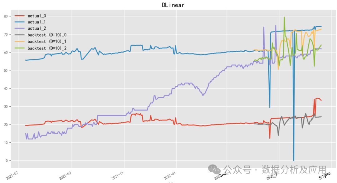
model = NHiTSModel(input_chunk_length=30, output_chunk_length=15, n_epochs=100, num_stacks=3, num_blocks=1, num_layers=2, dropout=0.1, activation='ReLU')2.4.9 D-Linear (2022)
Paper: Are Transformers Effective for Time Series Forecasting?
Code: https://github.com/cure-lab/LTSF-Linear
D-Linear (Deep Linear Model) is a neural network time series forecasting model meticulously crafted by the Hongyi Li team, which uses a linear approach to gain insights into time series data. It cleverly utilizes neural network structures for linear predictions, ensuring both high prediction accuracy and significantly enhancing the model’s interpretability. The model incorporates a multilayer perceptron architecture and continuously optimizes model performance through alternating training and fine-tuning strategies. Additionally, D-Linear innovatively proposes a feature selection mechanism based on sparse coding, intelligently filtering out features with discernibility and predictive value.