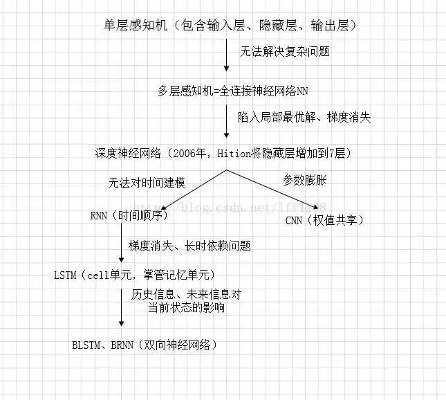
1. Introduction to CNN
CNN is a type of neural network that utilizes convolutional calculations. It can reduce the original image with very large pixel sizes to a smaller pixel image while retaining the main features. This article elaborates on the content from Professor Li Hongyi’s PPT.
1.1 Why CNN for Images
① Why Introduce CNN?
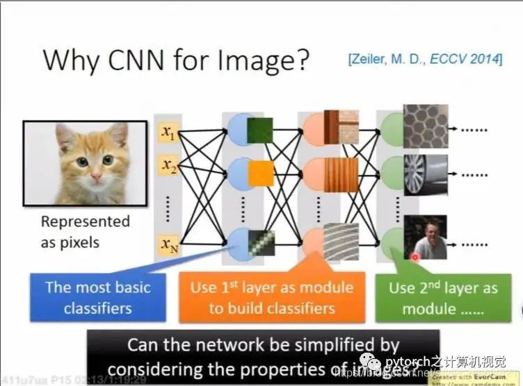
Image illustration: Given an image input to a fully connected neural network, the first hidden layer identifies whether the image contains green, yellow, or slanted stripes. The second hidden layer combines the outputs of the first hidden layer to achieve more complex functions. For example, if it sees a straight line + horizontal line, it is part of a frame; if it sees brown + stripes, it is wood grain; if it sees slanted stripes + green, it is part of gray stripes. Based on the output of the second hidden layer, if a certain neuron sees a beehive, it will activate; if it sees a person, it will activate.
However, if we use a fully connected neural network in a conventional way, we would need a lot of parameters. For example, if the input vector is 30,000 dimensions and the first hidden layer has 1,000 neurons, then the first hidden layer would require 30,000 * 1,000 parameters, resulting in a very large data volume, leading to low computational efficiency and accuracy. The introduction of CNN mainly addresses these issues by simplifying our neural network architecture. Certain weights are unnecessary, and CNN uses filtering methods to eliminate unneeded parameters while retaining important parameters for image processing.
② Why is it Sufficient to Use Fewer Parameters for Image Processing?
Three characteristics:
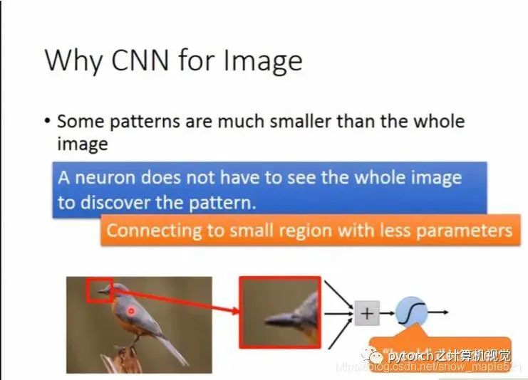
- Most patterns are smaller than the entire image. A neuron does not need to observe the entire image; it only needs to look at a small part of the image to find a desired pattern. For example, given an image, a certain neuron in the first hidden layer finds the bird’s beak, while another neuron finds the bird’s claws. As shown in the figure, it only needs to look at the red box and does not need to observe the entire image to find the bird’s beak.
-
Bird beaks at different positions only require training one parameter to recognize the beak, not separate training.
-
We can use sub-sampling to reduce the image size without changing the target image.
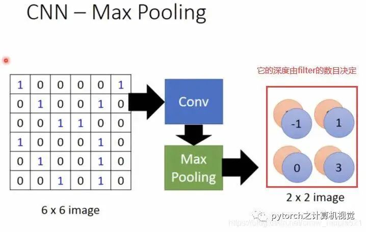
1.2 CNN Architecture Diagram
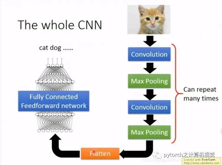
The first two properties in section 1.1 require convolutional calculations, while the last pooling layer processes them, which will be introduced in detail in the next section.
1.3 Convolutional Layer
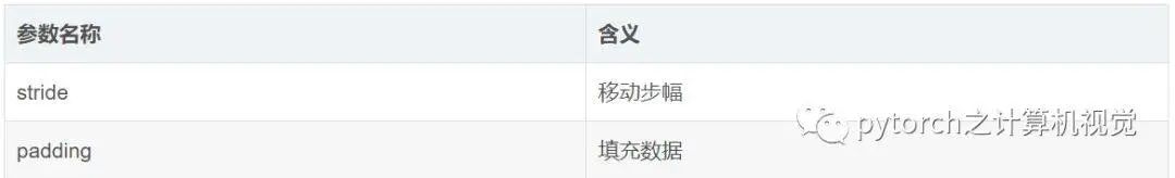
1.3.1 Important Parameters
1.3.2 Convolutional Calculation
The matrix convolution calculation is as follows:
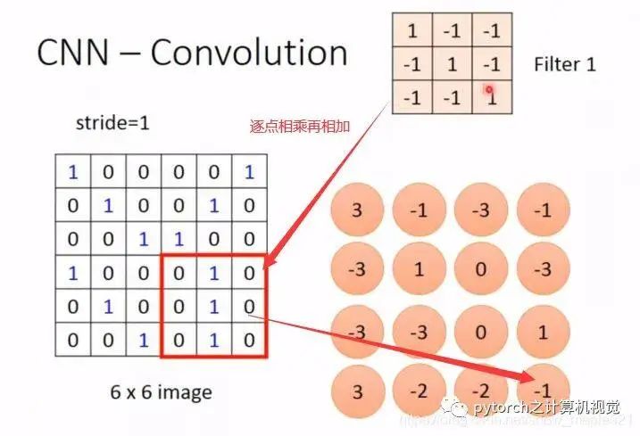
The calculation is as follows: the image input has pixel values of 553, and after padding = 1, it becomes pixel values of 773. The convolution kernel size is 333, with 2 convolution kernels and a stride of 2. Note that the depth of the convolution kernel must match the depth of the input pixel values. When the blue position of the scanned image corresponds to the red position of the convolution kernel, the multiplication and summation yield the data at the green position.
The pixel number changes to: (n + 2p – f) / s = (5 + 2 – 3) / 2 + 1 = 3, resulting in 332 data. The output pixel depth after convolution equals the number of convolution kernels from the previous layer. The resulting output is used as input for the pooling layer.
The size of the convolution kernel is often chosen as an odd number, and its depth must match the depth of the output pixel values from the previous layer. For example, the convolution kernel is chosen as 3*3*3, while the output pixel depth equals the number of convolution kernels in this convolution. Do not confuse this point.
1.3.3 Relationship Between Convolutional Layer and Fully Connected Layer
In fact, convolution simply removes some weights from the fully connected layer. The output of the convolutional layer is essentially the output from the hidden layer of the fully connected layer. As shown in the diagram:
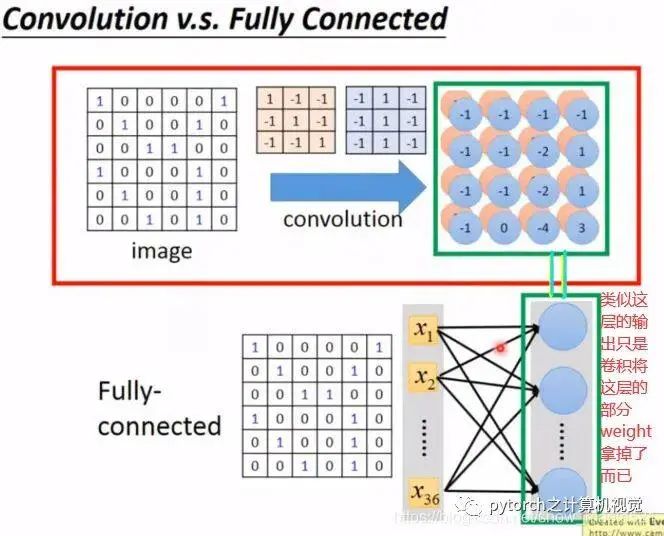
Convolution does not consider all features of the input; it only relates to the features passed through the filter. For example, a 6*6 image is unfolded into 36 pixels, and the next layer only relates to 9 pixels from the input layer, without connecting all pixels. This way, it uses very few parameters, as illustrated below:
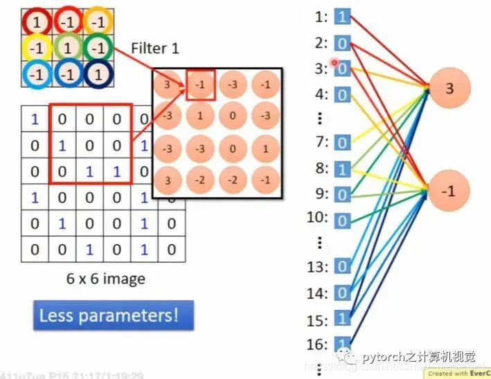
From the above diagram, we can see that the calculations for 3 and -1 do not require different weights like in a fully connected network; instead, the weights for these calculations are the same. This is known as weight sharing.
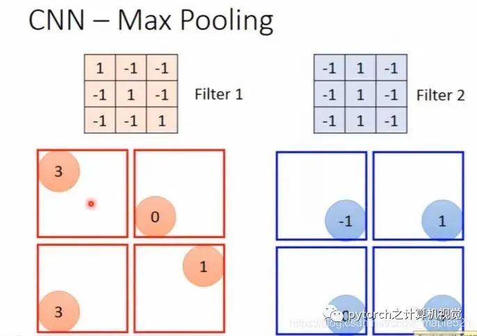
1.4 Pooling Layer
Based on the matrix from the previous convolution calculation, pooling is performed (merging four values within a box into one value, which can be the maximum or average value), as shown in the diagram:
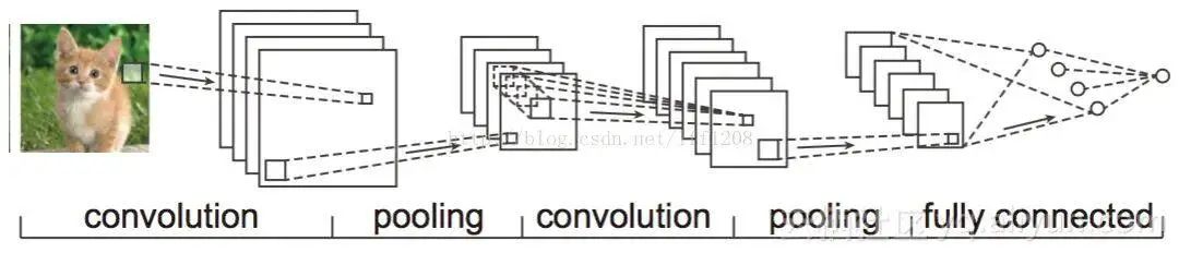
1.5 Applications
The PyTorch framework is mainly used to introduce convolutional neural networks.
Source code:
torch.nn.Conv2d(
    in_channels: int, # Number of input image channels
    out_channels: int, # Number of output channels produced by convolution
    kernel_size: Union[T, Tuple[T, T]], # Size of the convolution kernel
    stride: Union[T, Tuple[T, T]] = 1, # Stride of convolution, default: 1
    padding: Union[T, Tuple[T, T]] = 0, # 0-padding added to both sides of input, default: 0
    dilation: Union[T, Tuple[T, T]] = 1, # Spacing between kernel elements, default: 1
    groups: int = 1, # Number of blocked connections from input channels to output channels, default: 1
    # groups: controls the connections between input and output, the number of input and output channels must be divisible by groups,
    # when groups=1: all inputs are passed to all outputs
    # when groups=2: equivalent to two convolution layers, one sees half of the input channels and produces half of the output channels, merging both
    # when groups=in_channels: each channel has its own set of filters of size out_channel/in_channel
    bias: bool = True, # Adds a learnable bias to the output, default: true
    padding_mode: str = 'zeros')
# Note: kernel_size, stride, padding, dilation parameters can be int or tuple; when tuple, the first int is height dimension, the second is width dimension. When a single int, height and width values are the same.

# Square kernel and equal stride
m = nn.Conv2d(16, 33, 3, stride=2)
# Non-square kernel and unequal stride and padding
m = nn.Conv2d(16, 33, (3, 5), stride=(2, 1), padding=(4, 2))
# Non-square kernel and unequal stride and padding and dilation
m = nn.Conv2d(16, 33, (3, 5), stride=(2, 1), padding=(4, 2), dilation=(3, 1))
input = torch.randn(20, 16, 50, 100)
output = m(input)
Application: Here we use VGG16, and introduce the PyTorch torchsummary library, which can print the network model, for example:
import torchvision.models as models
import torch.nn as nn
import torch
from torchsummary import summary

device = torch.device('cuda' if torch.cuda.is_available() else 'cpu')

model = models.vgg16(pretrained=True).to(device)
print(model)
Output:
VGG(
  (features): Sequential(
    (0): Conv2d(3, 64, kernel_size=(3, 3), stride=(1, 1), padding=(1, 1))
    (1): ReLU(inplace)
    (2): Conv2d(64, 64, kernel_size=(3, 3), stride=(1, 1), padding=(1, 1))
    (3): ReLU(inplace)
    (4): MaxPool2d(kernel_size=2, stride=2, padding=0, dilation=1, ceil_mode=False)
    (5): Conv2d(64, 128, kernel_size=(3, 3), stride=(1, 1), padding=(1, 1))
    (6): ReLU(inplace)
    (7): Conv2d(128, 128, kernel_size=(3, 3), stride=(1, 1), padding=(1, 1))
    (8): ReLU(inplace)
    (9): MaxPool2d(kernel_size=2, stride=2, padding=0, dilation=1, ceil_mode=False)
    (10): Conv2d(128, 256, kernel_size=(3, 3), stride=(1, 1), padding=(1, 1))
    (11): ReLU(inplace)
    (12): Conv2d(256, 256, kernel_size=(3, 3), stride=(1, 1), padding=(1, 1))
    (13): ReLU(inplace)
    (14): Conv2d(256, 256, kernel_size=(3, 3), stride=(1, 1), padding=(1, 1))
    (15): ReLU(inplace)
    (16): MaxPool2d(kernel_size=2, stride=2, padding=0, dilation=1, ceil_mode=False)
    (17): Conv2d(256, 512, kernel_size=(3, 3), stride=(1, 1), padding=(1, 1))
    (18): ReLU(inplace)
    (19): Conv2d(512, 512, kernel_size=(3, 3), stride=(1, 1), padding=(1, 1))
    (20): ReLU(inplace)
    (21): Conv2d(512, 512, kernel_size=(3, 3), stride=(1, 1), padding=(1, 1))
    (22): ReLU(inplace)
    (23): MaxPool2d(kernel_size=2, stride=2, padding=0, dilation=1, ceil_mode=False)
    (24): Conv2d(512, 512, kernel_size=(3, 3), stride=(1, 1), padding=(1, 1))
    (25): ReLU(inplace)
    (26): Conv2d(512, 512, kernel_size=(3, 3), stride=(1, 1), padding=(1, 1))
    (27): ReLU(inplace)
    (28): Conv2d(512, 512, kernel_size=(3, 3), stride=(1, 1), padding=(1, 1))
    (29): ReLU(inplace)
    (30): MaxPool2d(kernel_size=2, stride=2, padding=0, dilation=1, ceil_mode=False)
  )
  (classifier): Sequential(
    (0): Linear(in_features=25088, out_features=4096, bias=True)
    (1): ReLU(inplace)
    (2): Dropout(p=0.5)
    (3): Linear(in_features=4096, out_features=4096, bias=True)
    (4): ReLU(inplace)
    (5): Dropout(p=0.5)
    (6): Linear(in_features=4096, out_features=1000, bias=True)
  )
)
model.classifier = nn.Sequential(
    *list(model.classifier.children())[:-1])    # remove last fc layer
print(model)
summary(model,(3,224,224))
Output:
----------------------------------------------------------------
        Layer (type)               Output Shape         Param #
================================================================
            Conv2d-1         [-1, 64, 224, 224]           1,792
              ReLU-2         [-1, 64, 224, 224]               0
            Conv2d-3         [-1, 64, 224, 224]          36,928
              ReLU-4         [-1, 64, 224, 224]               0
         MaxPool2d-5         [-1, 64, 112, 112]               0
            Conv2d-6        [-1, 128, 112, 112]          73,856
              ReLU-7        [-1, 128, 112, 112]               0
            Conv2d-8        [-1, 128, 112, 112]         147,584
              ReLU-9        [-1, 128, 112, 112]               0
        MaxPool2d-10          [-1, 128, 56, 56]               0
           Conv2d-11          [-1, 256, 56, 56]         295,168
             ReLU-12          [-1, 256, 56, 56]               0
           Conv2d-13          [-1, 256, 56, 56]         590,080
             ReLU-14          [-1, 256, 56, 56]               0
           Conv2d-15          [-1, 256, 56, 56]         590,080
             ReLU-16          [-1, 256, 56, 56]               0
        MaxPool2d-17          [-1, 256, 28, 28]               0
           Conv2d-18          [-1, 512, 28, 28]       1,180,160
             ReLU-19          [-1, 512, 28, 28]               0
           Conv2d-20          [-1, 512, 28, 28]       2,359,808
             ReLU-21          [-1, 512, 28, 28]               0
           Conv2d-22          [-1, 512, 28, 28]       2,359,808
             ReLU-23          [-1, 512, 28, 28]               0
        MaxPool2d-24          [-1, 512, 14, 14]               0
           Conv2d-25          [-1, 512, 14, 14]       2,359,808
             ReLU-26          [-1, 512, 14, 14]               0
           Conv2d-27          [-1, 512, 14, 14]       2,359,808
             ReLU-28          [-1, 512, 14, 14]               0
           Conv2d-29          [-1, 512, 14, 14]       2,359,808
             ReLU-30          [-1, 512, 14, 14]               0
        MaxPool2d-31            [-1, 512, 7, 7]               0
           Linear-32                 [-1, 4096]     102,764,544
             ReLU-33                 [-1, 4096]               0
          Dropout-34                 [-1, 4096]               0
           Linear-35                 [-1, 4096]      16,781,312
             ReLU-36                 [-1, 4096]               0
          Dropout-37                 [-1, 4096]               0
================================================================
Total params: 134,260,544
Trainable params: 134,260,544
Non-trainable params: 0
----------------------------------------------------------------
Input size (MB): 0.57
Forward/backward pass size (MB): 218.58
Params size (MB): 512.16
Estimated Total Size (MB): 731.32
----------------------------------------------------------------
2. Introduction to RNN
2.1 Introduction
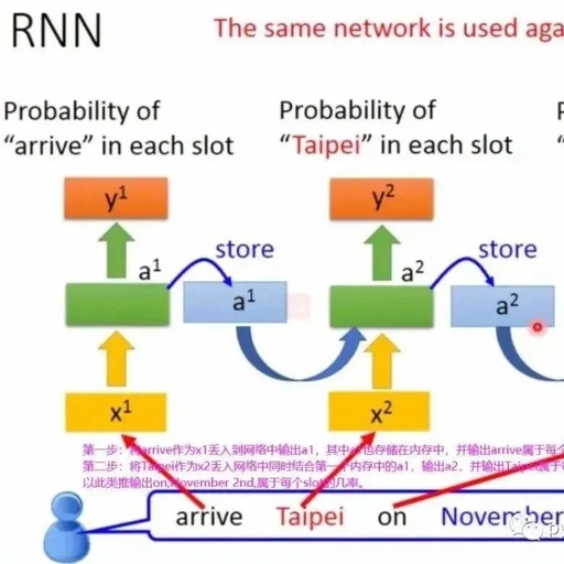
Every ticket booking system will have a slot filling mechanism. Some slots are for Destination, while some are for time of arrival; the system needs to know which words belong to which slot. For example:
I would like to arrive Taipei on November 2nd;
Here, Taipei is the Destination, November 2nd is the time of arrival;
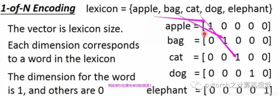
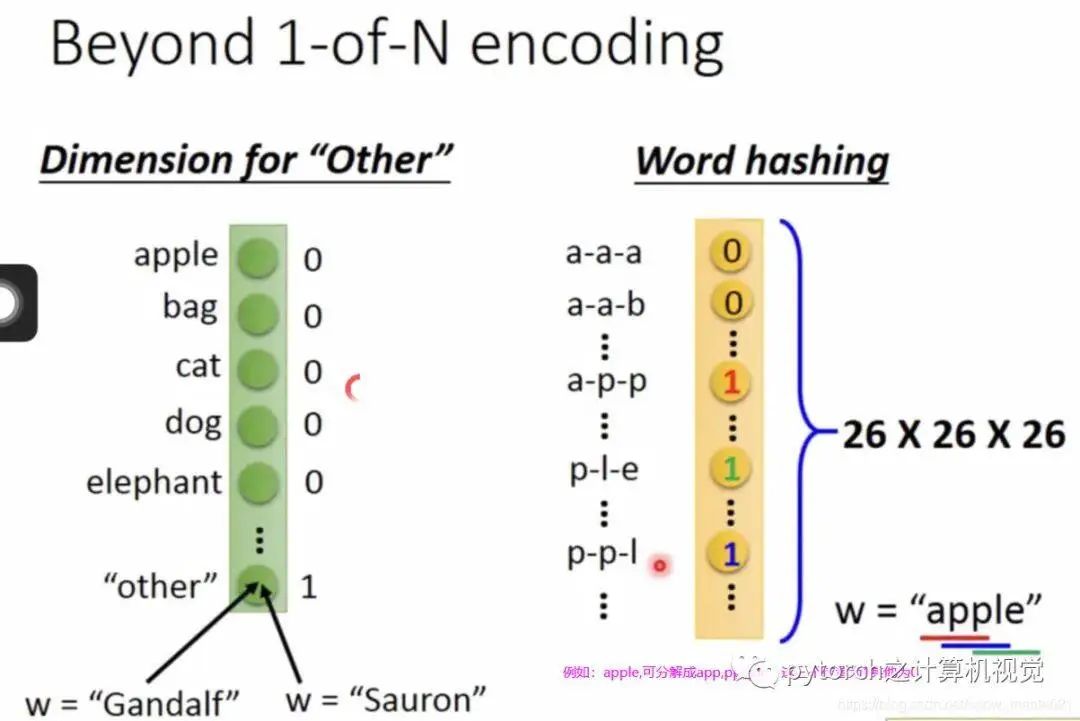
Using a regular neural network, we input the word Taipei into the network, but before inputting, we need to convert it into a vector representation. How to represent it as a vector? There are many methods; here we use: 1-of-N Encoding, represented as follows:
Other word vector methods are as follows:
However, if the following situation occurs, the system will make a mistake.
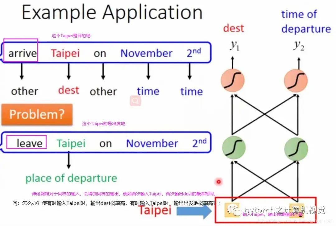
Question: What to do? Sometimes when inputting Taipei, the output probability for destination should be high, and sometimes when inputting Taipei, the output probability for departure should be high?
Answer: At this point, our network needs to have “memory” to remember the previously input data. For example, when Taipei is the destination, it sees the word arrive; when Taipei is the departure point, it sees the word leave. This memory-enabled network is called a Recurrent Neural Network (RNN).
2.2 Introduction to RNN
The output of the hidden layer of RNN is stored in memory, which will be used when the next input data comes in. The diagram is as follows:
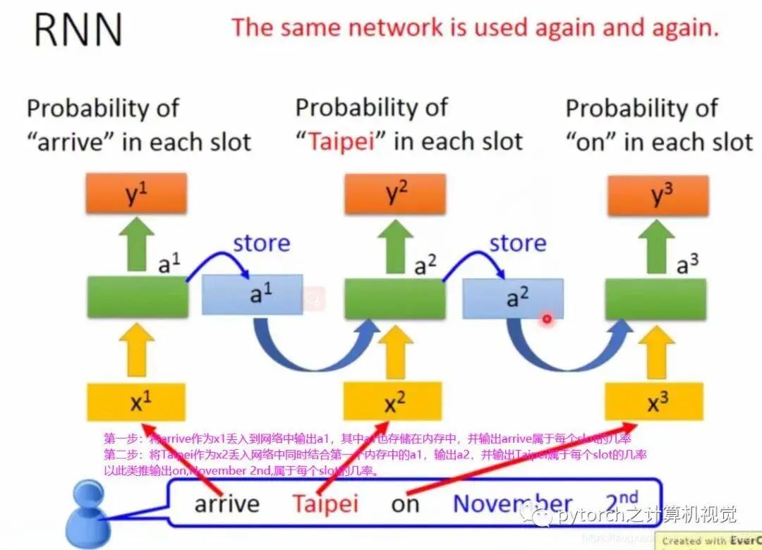
In the diagram, the same weights are represented by the same colors. Of course, the hidden layer can have many layers; the RNN introduced above is the simplest version, and the next section will introduce the enhanced version, LSTM.
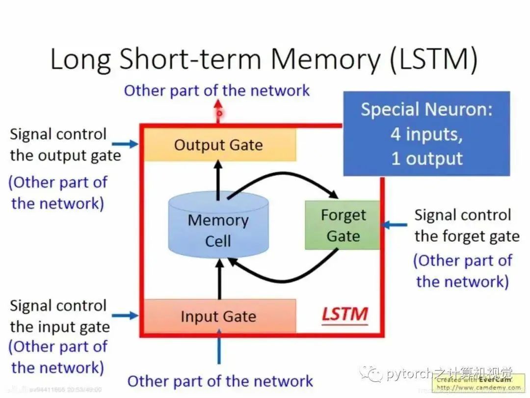
2.3 LSTM in RNN
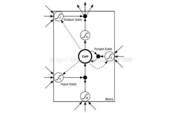
The commonly used memory is Long Short-Term Memory.
When external information needs to be input into memory, a “gate”—the input gate—is required, and when the input gate opens and closes is learned by the neural network. Similarly, the output gate is also learned by the neural network, as is the forget gate.
Thus, LSTM has four inputs and one output. A simplified diagram is as follows:
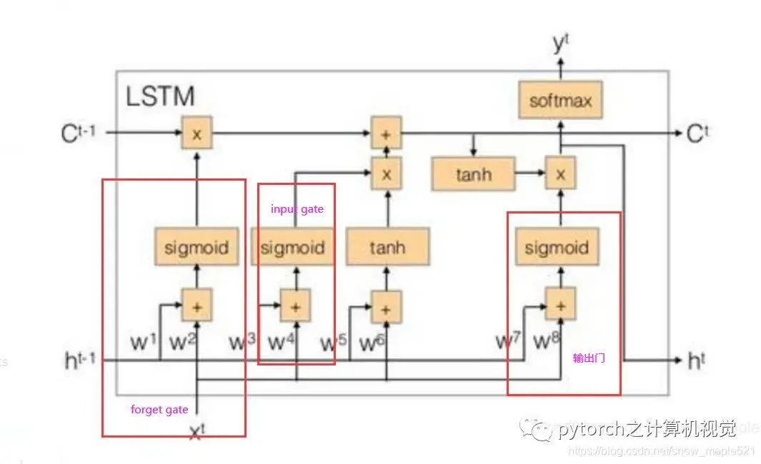
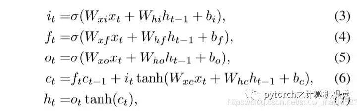
The formulas are as follows:
2.4 Example of LSTM
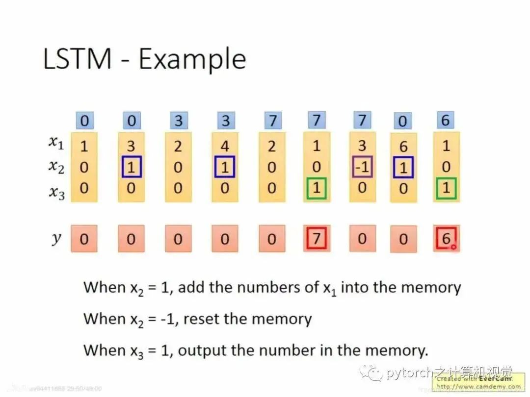
In the diagram, x2 = 1 sends x1 into memory; if x2 = -1, it clears the values in memory; if x3 = 1, it outputs the data from memory. As shown in the diagram, in the first column, x2 = 0 does not send anything to memory; in the second column, x2 = 1 sends the current x1 = 3 into memory (note that the data in memory is accumulated, for example, in the fourth column, x2 = 1, at this time x1 = 4, memory = 3, so the total is 7). In the fifth column, x3 = 1, which allows output, so it outputs the value of memory, which is 7.
Combining the simplified diagram of LSTM:
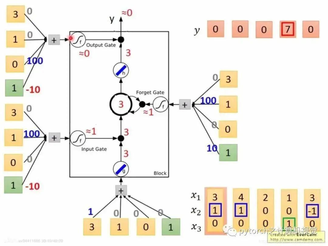
Assuming the first column input is: x1 = 3, x2 = 1, x3 = 0, the steps are: g—Tanh: x1w1 + x2w2 + x3w3 = 3, f—sigmoid: x1w1 + x2w2 + x3w3 = 90, after sigmoid = 1, after calculating f and g, input gate = 3*1 = 3, forget gate = 1, meaning no need to clear, x3 = 0 indicates the output gate is locked, so the output remains 0.
2.5 Practical LSTM
In PyTorch, the LSTM network is encapsulated and can be directly used with nn.LSTM, for example:
class QstEncoder(nn.Module):

    def __init__(self, qst_vocab_size, word_embed_size, embed_size, num_layers, hidden_size):

        super(QstEncoder, self).__init__()
        self.word2vec = nn.Embedding(qst_vocab_size, word_embed_size)
        self.tanh = nn.Tanh()
        self.lstm = nn.LSTM(word_embed_size, hidden_size, num_layers)
        self.fc = nn.Linear(2*num_layers*hidden_size, embed_size)     # 2 for hidden and cell states
    def forward(self, question):

        qst_vec = self.word2vec(question)                             # [batch_size, max_qst_length=30, word_embed_size=300]
        qst_vec = self.tanh(qst_vec)
        qst_vec = qst_vec.transpose(0, 1)                             # [max_qst_length=30, batch_size, word_embed_size=300]
        _, (hidden, cell) = self.lstm(qst_vec)                        # [num_layers=2, batch_size, hidden_size=512]
        qst_feature = torch.cat((hidden, cell), 2)                    # [num_layers=2, batch_size, 2*hidden_size=1024]
        qst_feature = qst_feature.transpose(0, 1)                     # [batch_size, num_layers=2, 2*hidden_size=1024]
        qst_feature = qst_feature.reshape(qst_feature.size()[0], -1)  # [batch_size, 2*num_layers*hidden_size=2048]
        qst_feature = self.tanh(qst_feature)
        qst_feature = self.fc(qst_feature)                            # [batch_size, embed_size]

        return qst_feature
3. Differences Between CNN and RNN
The differences between CNN and RNN are summarized in the following link, referencing the summary by the blog author (https://blog.csdn.net/lff1208/article/details/77717149):
DNN Formation
To overcome gradient vanishing, ReLU, maxout, etc., are used as activation functions instead of sigmoid, forming the basic form of today’s DNN. The structure is similar to that of a multilayer perceptron, as shown in the diagram:
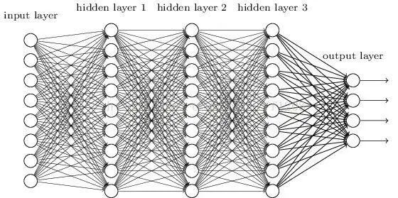
We see that in the structure of fully connected DNN, lower-layer neurons can connect to all upper-layer neurons, leading to an explosion in the number of parameters. Assuming the input is an image with pixel size of 1K*1K and the hidden layer has 1M nodes, just this layer would require 10^12 weights to be trained, which not only easily leads to overfitting but also easily falls into local optima.
CNN Formation
Due to the inherent local patterns in images (such as eyes, nose, mouth in a face), convolutional neural networks (CNN) emerged by combining image processing with neural networks. CNN connects upper and lower layers through convolutional kernels, with the same convolution kernel shared across all images, preserving the original positional relationships after convolution.
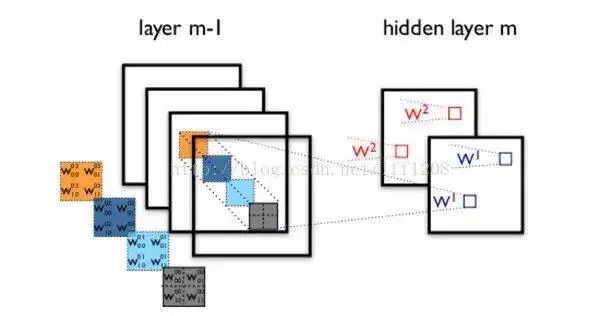
To illustrate the structure of convolutional neural networks, let’s say we need to recognize a color image, which has four channels ARGB (transparency and red, green, blue corresponding to four images of the same size). Assuming the convolution kernel size is 100*100, and we use 100 convolution kernels from w1 to w100 (intuitively, each convolution kernel should learn different structural features).
Using w1 on the ARGB image for convolution will yield the first image in the hidden layer; the upper left pixel of this hidden layer image is the weighted sum of the pixels in the upper left 100*100 area of the four input images, and so on.
Similarly, considering other convolution kernels, the hidden layer corresponds to 100 “images”. Each image responds to different features in the original image. This structure continues to propagate. CNN also includes operations like max-pooling to further enhance robustness.
Note that the last layer is actually a fully connected layer; in this example, we note that the number of parameters from the input layer to the hidden layer has instantly reduced to 100*100*100 = 10^6! This allows us to obtain a good model using the existing training data. The statement that applies to image recognition is precisely because the CNN model limits the number of parameters and exploits the characteristics of local structures. Following the same reasoning, CNN can also be applied to speech recognition by utilizing local information in the speech spectrogram structure.
RNN Formation
DNN cannot model changes over time sequences. However, the temporal order of sample appearances is crucial for applications such as natural language processing, speech recognition, and handwriting recognition. To meet this demand, another type of neural network structure has emerged—Recurrent Neural Network (RNN).
In ordinary fully connected networks or CNNs, the signals from each layer of neurons can only propagate upward, and the processing of samples at various moments is independent; thus, they are also called feed-forward neural networks. In RNN, the output of neurons can directly affect themselves in the next time period. That is, the input of the i-th layer neuron at time m includes not only the output of the (i-1)-th layer neuron at that time but also its own output at (m-1)! This can be represented in a diagram as follows:
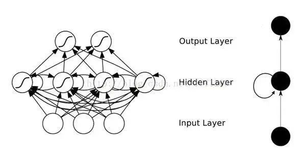
For convenience in analysis, the following diagram unfolds according to time periods:
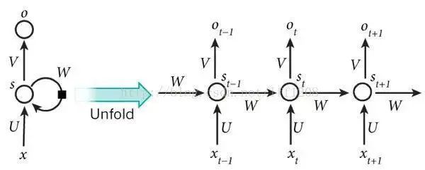
The final result O(t+1) of the network at time (t+1) is the result of the input at that moment combined with all historical inputs! This achieves the purpose of modeling time series. RNN can be seen as a neural network that transmits over time, where its depth is the length of time! As we mentioned earlier, the “gradient vanishing” phenomenon will occur again, but this time along the time axis.
Thus, RNN has the problem of being unable to solve long-term dependencies. To address this issue, LSTM (Long Short-Term Memory) was proposed, which implements memory functions over time through cell gate switches and prevents gradient vanishing. The structure of the LSTM unit is shown in the diagram below:
In addition to DNN, CNN, RNN, ResNet (Deep Residual), and LSTM, there are many other types of neural network structures. For instance, in sequence signal analysis, if I can predict the future, it will also help with recognition. Hence, bidirectional RNN and bidirectional LSTM have emerged, utilizing both historical and future information.
In fact, regardless of the type of network, they are often mixed in practical applications. For example, CNN and RNN often connect to a fully connected layer before outputting, making it hard to categorize a specific network into a single category. It is not difficult to imagine that as the popularity of deep learning continues, more flexible combinations and diverse network structures will be developed.
In summary: